Download
1 / 55
550 likes | 724 Views
References. Book : Andrew N. Cleland, Foundation of Nanomechanics Springer,2003 (Chapter7,esp.7.1.4, Chapter 8,9); Reviews: R.Shekhter et al. Low.Tepmp.Phys . 35, 662 (2009); J.Phys . Cond.Mat . 15, R 441 (2003)

E N D
References Book: Andrew N. Cleland, Foundation of Nanomechanics Springer,2003 (Chapter7,esp.7.1.4, Chapter 8,9); Reviews:R.Shekhter et al. Low.Tepmp.Phys. 35, 662 (2009); J.Phys. Cond.Mat. 15, R 441 (2003) J. Comp.Theor.Nanosc., 4, 860 (2007)
Five-Lecture Course on the Basic Physics of Nanoelectromechanical Devices • Lecture 1: Introduction to nanoelectromechanical systems (NEMS) • Lecture 2: Electronics and mechanics on the • nanometer scale • Lecture 3: Mechanically assisted single electronics • Lecture 4: Quantum nano-electro-mechanics • Lecture 5: Superconducting NEM devices
Lecture 2: Electronics and Mechanics on the Nanometer Scale Outline • Electronics – Mesoscopic phenomena • Mechanics - Classical dynamics of mechanical deformations
Lecture 2: Electronics and Mechanics on the Nanometer Scale Part 1Electronics – Mesoscopic phenomena
Lecture 2: Electronics and Mechanics on the Nanometer Scale Mesosopic phenomena • Persistent currents (in the ground state) • Microscopic scale: Electrons move in atomic orbitals, • may generate net magnetization • Macroscopic scale: No current in the ground state of bulk sample • Mesoscopic scale: Persistent currents in the ground state • Coulomb blockade (due to discreteness of electronic charge) • Microscopic scale: Electrons have finite charge e, Coulomb interactions • give rise to large ionization energies of atoms • Macroscopic scale: Electron liquid, charge discreteness not important • Mesoscopic scale: Coulomb blockade of tunneling through granular samples • Josephson effect (supercurrent passing through NS-region) • A supercurrent may flow between two superconductors separated by a • non-superconducting region of mesoscopic size Mesoscopic samples contain a large number of atoms but are small on the scale of a temperature-dependent ”coherence length”. On such scales electronic and mechanical phenomena coexist: Mesoscopic Nanoelectromechanics
Lecture 2: Electronics and Mechanics on the Nanometer Scale Quantum Coherence of Electrons • Spatial quantization of electronic motion • Quantum tunneling of electrons • Resonance transmission phenomenon • Tunnel charge relaxation and tunnel resistance
Lecture 2: Electronics and Mechanics on the Nanometer Scale 7/48 Spatial quantization of orbital motion • For a sample with symmetric shape the electronic spectrum is degenerate • A distortion of the geometrical shape tends to lift degeneracies.
Lecture 2: Electronics and Mechanics on the Nanometer Scale Quantum Level Spacing Estimation of average level spacing, assuming all quantum states are nondegenerate and homogeneously distributed in energy N – total number of electrons
Lecture 2: Electronics and Mechanics on the Nanometer Scale Quantum Tunneling The classically moving electron is reflected by a potential barrier and can not be “seen” in the region x > 0. The quantum particle can penetrate into such a forbidden region. Under-the-barrier propagation: Under-the-barrier propagation is calledtunneling. Wave function’s decay length is called the tunneling length.
Lecture 2: Electronics and Mechanics on the Nanometer Scale Tunneling through a Barrier Due to quantum tunneling a particle has a finite probability to penetrate through a barrier of arbitrary height. t and r are probability amplitudes for the transmission and reflection of the particle. These parameters characterise the barrier and can often be considered to be only weakly energy dependent.
Lecture 2: Electronics and Mechanics on the Nanometer Scale Tunneling Width of a Quantum Level Let N be the number of ”tries” made before the particle finally escapes the dot: Escape time
Lecture 2: Electronics and Mechanics on the Nanometer Scale Resonant Tunneling Electronic waves, like ordinary waves, experience a set of multiple reflections as they move back and forth between two barriers. The total probability amplitude for the transfer of a particle can be viewed as a sum of amplitudes, each corresponding to escape after an increasing number of “bounces” between the barriers. If p = pn = nh/2d we have D=1 independently of the barrier transparency! (Resonance) Breit-Wigner formula
Lecture 2: Electronics and Mechanics on the Nanometer Scale Tunneling Resistance L An electric field must be present in the vicinity of the barrier in order to compensate for the ”scattering force” of the potential barrier and achieve a stationary current flow The resulting voltage drop across the barrier, V = eEL, determines the tunneling resistance, R = V/I
Lecture 2: Electronics and Mechanics on the Nanometer Scale Quantization Effects in Electronic Tanspansport Conductance of a quantum point contact: Adiabatic point cointact Landauer formula
Lecture 2: Electronics and Mechanics on the Nanometer Scale Charge Relaxation Due to Tunneling Q -Q If one transfers a charge Q from one conductor to the other, it will first accumulate in surface layers on both sides of the tunnel barrier, and will then relax due to tunneling of electrons .
Lecture 2: Electronics and Mechanics on the Nanometer Scale Characteristic Energy Scales (summary) Level spacing: 0.1-1 K Level width: 0.01-0.1 K Frequency of tunnel charge relaxation : 0.01-0.1 K d= 1-10nm D=0.0001 At low enough temperatures all quantum coherent effects might be experimentaly relevant.
Lecture 2: Electronics and Mechanics on the Nanometer Scale Tunnel Transport of Discrete Charges • Charge transport in granular conductors is entirely due to tunneling of electrons between small neighboring conducting grains. • The electronic charge on each of the grains is quantized in units of the elementary electronic charge. • This results in quantization of the electrostatic energy, which may block the intergrain tunneling of electrons.
Lecture 2: Electronics and Mechanics on the Nanometer Scale Single Electron Transistor V/2 -V/2 - Mutual capacitances e e Source Drain Gate
As a result, Lecture 2: Electronics and Mechanics on the Nanometer Scale
(Master equation) Lecture 2: Electronics and Mechanics on the Nanometer Scale I-V curves: Coulomb staircase g e c How one can calculate the I-V curve? - +
Conductance oscillates as a function of gate voltage – Coulomb blockade oscillations. Lecture 2: Electronics and Mechanics on the Nanometer Scale Stability Diagram for a Single-Electron Transistor Coulomb diamonds: all transfer energies inside are positive.
V=10 μV Lecture 2: Electronics and Mechanics on the Nanometer Scale Experimental test: Al-Al203 SET, temperature 30 mK Coulomb blockade oscillations
Thermal smearing Experiment: STM of surface clusters Coulomb staircase Calculations for different gate potentials Lecture 2: Electronics and Mechanics on the Nanometer Scale Coulomb Staircase
Lecture 2: Electronics and Mechanics on the Nanometer Scale Single-Electron Transistor Device SETs are promising for logical operations since they manipulate by single electrons, and this is why have low power consumption per bit. The operation temperature is actually set by the relationship between the charging energy, Ec=e2/2C, and the thermal smearing, kΘ. At present time, room-temperature operation has been demonstrated. Coulomb blockade and single-electron effects are specifically important for molecular electronics, where the size is intrinsically small. Negative feature of SETs is their sensitivity to fluctuations of the background charges.
Lecture 2: Electronics and Mechanics on the Nanometer Scale Submicron SET Sensors • CB primary termometer (based on thermal smearing of the CB) in the range 20 mK - 50 K (dT~3%) • (J.Pekkola, J.LowTemp.Phys. 135, (2004), T. Bergsten et al. Appl.Phys.Lett. 78, 1264 (2001)) • Most sensitive electrometers (based on SET being sensitive to the gate potential Vg): dq ~ 10-6 eHz-1/2 • (M.Devoret et al., Nature 406, 1039 (2000)). • CB current meter (based on SET oscillations in the time domain) • (J.Bylander et al. Nature 434, 361 (2005) )
Lecture 2: Electronics and Mechanics on the Nanometer Scale Quantum Fluctuation of Electric Charge Charge fluctuations due to quantum tunneling smear the charge quantization . This destroys the Coulomb Blockade. Coulomb Blockade is destroyed by quantum fluctuations of thecharge Coulomb Blockade is restored
Lecture 2: Electronics and Mechanics on the Nanometer Scale Part 2.Mechanics – Classical Dynamics of Mechanical Deformations
Lecture 2: Electronics and Mechanics on the Nanometer Scale Mechanical Dynamics of Nanostructures Focus on spatial displacements of bodies and their parts Examples F F m F Motion of a point-like mass Rotational displacement + center-of-mass motion Elastic deformations Displacements: Classical and Quantum The discrete nature of solids can be ignored on the nanometer length scale
Lecture 2: Electronics and Mechanics on the Nanometer Scale Classical Mechanics of a Point-Like Mass Newton’s equation In most cases we may consider to be of elastic or electric origin Classical harmonic oscillator: U x
Lecture 2: Electronics and Mechanics on the Nanometer Scale Euler-Bernoulli Equation P(x) U(x) E – Young’s modulus – represents rigidity of the material I – Second moment of crossection – represent influence of the crossectional geometry Why there is sensitivity to geometry of the beam crossection? Easy to bend Dificult to bend
Lecture 2: Electronics and Mechanics on the Nanometer Scale Longitudinal and Flexural Vibrations Londitudinal elastic vibrations Flexural vibrations Longitudinal deformation: Compression across the whole crossection Flexural deformation. Compression and streching occur at different parts of the crossection
Lecture 2: Electronics and Mechanics on the Nanometer Scale Flexural Vibrations of a Strained Beam APL 78 (2001) 162
Lecture 2: Electronics and Mechanics on the Nanometer Scale Flexural Vibrations of a Doubly Clamped Beam Ref: A.N. Cleland, Foundations of Nanoelectromechanics (Springer, 2003), Ch. 7 Nanotube: L=100nm, d=1.4 nm, f0=5 GHz A: cross-section area (=HW) ρ: mass density of the beam E,I: assumed independent of position The solution is: Silicon: L=1mm, H=W=0.1 mm, f0=1 GHz
Lecture 2: Electronics and Mechanics on the Nanometer Scale Flexural Vibrations of a Cantilever Ref: A.N. Cleland, Foundations of Nanoelectromechanics (Springer, 2003) A: cross-section area (=HW) ρ: mass density of the beam E,I: assumed independent of position The solution is:
Lecture 2: Electronics and Mechanics on the Nanometer Scale Damping of the Mechanical Motion • So far we have ignoredanyinteraction of the mechanical vibrations with the manyother degrees of freedom present in the solid. Eventhoughsuchinteractionsmay be relativelyweaktheycould produce a significant effect on a largeenough time scale. The interactions cause dissipation of the mechanicalenergy and stochasticdeviations from the otherwise regular mechanical vibrations (noise). • Sources of dissipation and noise are the same and might come from: • Interaction with other mechanical modes • Interaction with electrons • (nonintrinsic source) motion of defects and ions due to imposed strain. • Interaction with a suface contaminations • Below we will present a phenomenological approach to describe these effects without going into the microscopic theory for any particular mechanism.
Lecture 2: Electronics and Mechanics on the Nanometer Scale Dissipation and Noise in Mechanical Systems Ref: A.N. Cleland, Foundations of Nanoelectromechanics (Springer, 2003), Ch. 8 Outline • Langevin Equation (useful phenomenological approach) • Dissipation and Quality Factor • Dissipation in Nanoscale Mechanical Resonators • - Dissipation-Induced Amplitude Noise Einstein (1905 – ”annus mirabulis”): Friction and Brownian motion is connected; where there is dissipation there is also noise
Lecture 2: Electronics and Mechanics on the Nanometer Scale Langevin Equation Consider a system of inertial mass m that interacts with its environment through a conservative potentialU(x)=kx2/2 +... and in addition through a complex interaction term characterized both by friction and noise. Without friction the dynamic equation is Newton’s equation which has a lossless solution x(t)wherex0andφare determined by the initial conditions: Friction and noise in the system is due to the interaction of the mass m with a large number of degrees of freedom in the environ- ment. It can be included by adding a time-dependent environmental force term to Newton’s equation Paul Langevin (1872-1946)
Lecture 2: Electronics and Mechanics on the Nanometer Scale Dissipation and Noise are Due to the Environment In many dissipative systems the environmental force can be separated into a dissipation (or loss) term proportional to the ensemble average velocity and a noise term due to a random force Equations of this form are known as Langevin equations. The dissipative term in the Langevin equation causes energy to be transferred from the harmonic oscillator to the environment. Thermal equilibrium in a system controlled by the Langevin equation is achieved through the second moment of the noise force, which must satisfy:
Lecture 2: Electronics and Mechanics on the Nanometer Scale Dissipation and Environmental Noise Drives the System to Equilibrium and Maintains Equilibrium The mean energy of a harmonic oscillator is The energy of an undriven harmonic oscillator described by our Langevin equation will equilibriate to the energy of the environment by losing any initial excess energy to the environment by the velocity-dependent dissipation term and then, gaining and losing energy stochastically through the noise term the noise force will produce this equilibrium. Without proof we state that:
Lecture 2: Electronics and Mechanics on the Nanometer Scale Fundamental Relation between Environmental Noise, Dissipation and Temperature (Einstein 1905) If we assume that the noise force is uncorrelated for time scales over which the harmonic oscillator responds, we have so called white noise, and We can define a spectral density for the (noise) force-force correlation function as: For white noise the spectral density is constant (independent of frequency): Noise Dissipation Temperature
Lecture 2: Electronics and Mechanics on the Nanometer Scale Dissipation and Quality Factor (Q) In the absence of the noise term the solution to the Langevin equation is x(t)=x0exp(-iωt+φ), where the complex-valued frequency is given by The frequency ω has both real and imaginary parts, ω = ωR + i ωI: The quality factor Q is defined as:
Lecture 2: Electronics and Mechanics on the Nanometer Scale Damping of Mechanical Oscillations Now, since the oscillation amplitude damps as and the energy damps as
Lecture 2: Electronics and Mechanics on the Nanometer Scale Dissipation in Nanoscale Mechanical Resonators Recall the Euler-Bernoulli equation: A: cross-section area (=HW) ρ: mass density of the beam And its solution The imaginary part of w’n indicates that the n:th eigenmode will decay in amplitude as exp(-wn/2Q), similar to the damped harmonic oscillator Different with dissipation!
Lecture 2: Electronics and Mechanics on the Nanometer Scale Driven Damped Beams We add a harmonic driving forceF(x,t)=f(x)exp(-iwct), where f(x) is a position- dependent force per unit length and wc is the drive – or carrier – frequency. The equation of motion is now: Solve this for times longer than the damping time for the beam by expansion in terms of eigenfunctions: The equation for the expansion coefficients an is
Lecture 2: Electronics and Mechanics on the Nanometer Scale Using the definitions of the eigenfunctions and their properties, and the definition of the complex-valued eigenfrequenciesw’n this can be written as: For w close to w1, only the n=1 term has a significant amplitude, given by: For a uniform force distribution, f(x)=f0 , the integral is evaluated to 1L2, 1=0.8309 and we have, since w’n=(1-i/Q)wn:
Lecture 2: Electronics and Mechanics on the Nanometer Scale Dissipation-Induced Amplitude Noise The displacement of a forced damped beam driven near its fundamental frequence is – as we have seen – given by In the absence of noise the motion is purely harmonic at the carrier frequency w. But if there is dissipation (finiteQ), there is also necessarily noise and a noise force fN(t) that can be expanded in terms of the eigenfunctions un(x): As we discussed already dissipation drives the beam to equilibrium with its environment at temperature T and the stochastic noise force maintains the equilibrium.
Lecture 2: Electronics and Mechanics on the Nanometer Scale Without driving force the mean total energy for each mode is kBT. This requires the spectral density of the noise force fN,n(t) to be: Force per length, hence the term L2, which is not there for a simple harmonic osc. Using this result we can calculate the spectral density for the thermally driven amplitude as