Download
1 / 13
130 likes | 231 Views
Lecture 4 Measurement. Accuracy and Statistical Variation. Accuracy vs. Precision. Expectation of deviation of a given measurement from a known standard Often written as a percentage of the possible values for an instrument Precision is the expectation of deviation of a set of measurements

E N D
Lecture 4 Measurement Accuracy and Statistical Variation
Accuracy vs. Precision • Expectation of deviation of a given measurement from a known standard • Often written as a percentage of the possible values for an instrument • Precision is the expectation of deviation of a set of measurements • “standard deviation” in the case of normally distributed measurements • Few instruments have normally distributed errors
Deviations • Systematic errors • Portion of errors that is constant over data gathering experiment • Beware timescales and conditions of experiment– if one can identify a measurable input parameter which correlates to an error – the error is systematic • Calibration is the process of reducing systematic errors • Both means and medians provide estimates of the systematic portion of a set of measurements
Random Errors • The portion of deviations of a set of measurements which cannot be reduced by knowledge of measurement parameters • E.g. the temperature of an experiment might correlate to the variance, but the measurement deviations cannot be reduced unless it is known that temperature noise was the sole source of error • Error analysis is based on estimating the magnitude of all noise sources in a system on a given measurement • Stability is the relative freedom from errors that can be reduced by calibration– not freedom from random errors
Quantization Error • Deviations produced by digitization of analog measurements • For random signal with uniform quantization of xlsb: +lsb/2 x -lsb/2
Test Correlation • Tester to Bench • Tester to Tester • DIB to DIB • Day to Day • Goal is reproducible measurements within expected error magnitude
Model based Calibration • Given a set of accurate references and a model of the measurement error process • Estimate a correction to the measurement which minimizes the modeled systematic error • E.g. given two references and measurements, the linear model:
Multi-tone Calibration • DSP testing often uses multi-tone signals from digital sources • Analog signal recovery and DIB impedance matching distort the signal • Tester Calibration can restore signal levels • Signal strength usually measured as RMS value • Corresponds to square-law calibration fixture • Modeling proceeds similarly to linear calibration as long as the model is unimodal. In principle, any such model can be approximated by linear segments, and each segment inverted to find the calibration adjustment.
Noise Reduction: Filtering • Noise is specified as a spectral density (V/Hz1/2) or W/Hz • RMS noise is proportional to the bandwidth of the signal: • Noise density is the square of the transfer function • Net (RMS) noise after filtering is:
Filter Noise Example • RC filtering of a noisy signal • Assume uniform input noise, 1st order filter • The resulting output noise density is: • We can invert this relation to get the equivalent input noise:
Averaging (filter analysis) • Simple processing to reduce noise – running average of data samples • The frequency transfer function for an N-pt average is: • To find the RMS voltage noise, use the previous technique: • So input noise is reduced by 1/N1/2
‘Normal’ Statistics • Mean • Standard Deviation • Note that this is not an estimate for a total sample set (issue if N<<100), use 1/(N-1) • For large set of data with independent noise sources the distribution is: • Probability
Issues with Normal statistics • Assumptions: • Noise sources are all uncorrelated • All Noise sources are accounted for • In many practical cases, data has ‘outliers’ where non-normal assumptions prevail • Cannot Claim small probability of error unless sample set contains all possible failure modes • Mean may be poor estimator given sporadic noise • Median (middle value in sorted order of data samples) often is better behaved • Not used often since analysis of expectations are difficult