Download
1 / 37
370 likes | 502 Views
Modeling Generation Capacity Investment Decisions. GridSchool 2010 March 8-12, 2010 Richmond, Virginia Institute of Public Utilities Argonne National Laboratory Vladimir Koritarov Center for Energy, Economic, and Environmental Systems Analysis Decision and Information Sciences Division

E N D
Modeling Generation Capacity Investment Decisions GridSchool 2010 March 8-12, 2010 Richmond, Virginia Institute of Public Utilities Argonne National Laboratory Vladimir Koritarov Center for Energy, Economic, and Environmental Systems Analysis Decision and Information Sciences Division ARGONNE NATIONAL LABORATORY koritarov@anl.gov 630.252.6711 Do not cite or distribute without permission MICHIGAN STATE UNIVERSITY
Resource Planning Methodologies • Screening Curves • A comparison of annualized costs of different generating technologies across a range of capacity factors • Deterministic Optimization Models: • Optimization models using linear programming (LP) and/or mixed-integer programming (MIP) • Representative models: MARKAL, MESSAGE, etc. • Dynamic Programming Optimization Models: • Typically include a detailed dispatch model and a dynamic programming (DP) model • Provide a rigorous capacity expansion solution by examining thousands of possible future expansion paths • Representative models: WASP, EGEAS, etc. • New Methods for Deregulated electricity markets (e.g., Agent-Based Modeling): • Applicable in competitive electricity markets • Simulate independent decision-making of market participants • May not provide least-cost solution for the system as a whole
Screening Curves Provide a Simplified Approach for Quick Analysis of Economic Competitiveness • Separate technology costs into “fixed” and “variable” costs • Construct cost curves for each technology • Plot cost ($/kW-yr) vs. capacity factor • Determine least-cost alternatives as a function of utilization • Numerous limitations • Not a substitute for a thorough analysis
Total Annualized Cost ($/kW-yr) Annualized Fixed Cost ($/kW-yr) = + Variable Cost ($/kWh) × Capacity Factor (fraction) 8760 (h/yr) × Total Annualized Cost Includes Fixed and Variable Components Annualized Cost Variable Cost ($ / kW-yr) Fixed Cost Capacity Factor
Screening Curves Show Ranges of Competitiveness for each Technology
The Competitiveness of Certain Technologies is Sensitive to the Choice of Discount Rate 5% Discount Rate 10% Discount Rate
200 Coal (600 MW) Gas (50 MW) Nuclear (1000 MW) Total Annualized Fixed and Variable Cost ($ / kW-yr) .0635 .4866 0 0 1.0 Capacity Factor 1.0 Gas Turbine (.1311) .8689 Coal (.2327) .6362 Normalized Load (fraction) Nuclear (.6362) 0 0 1.0 Time (fraction) Lowest Cost Options Can be Projected onto a LDC to Obtain an Estimate of Supply Mix
The Screening Curve Approach Does Not Consider Many Important Factors in System Planning Screening curves do NOT consider: • Unit availability (forced outage and maintenance) • Existing capacity • Unit dispatch factors (minimum load and spinning reserve) • System reliability • Dynamic factors changing over time (load growth and economic trends) • Etc.
Deterministic Optimization Models • Relatively simple, easy to understand approach • The solution is obtained fast, in a single model run • The input data requirements are lower than for the dynamic programming optimization models • Can be computationally intensive if applied to real power systems (large number of variables and constraint equations require powerful solvers) • Dispatch model is rather simple, usually on an annual basis. Some models use 2 or even 5-year time step. • Numerous limitations in modeling system operation (e.g., no planned maintenance schedule) • Inadequate reliability analysis (typically planning reserve margins and energy-not-served (ENS) are calculated). • The ENS calculation is inaccurate due to simplified dispatch • The optimal solution may not be feasible or realistic • The LP solution does not consider discrete unit sizes (not all models have MIP capabilities)
Energy Reserves/ Resources Example: Oil, natural gas, or coal reserves (billion tons) Primary Energy Production Crude oil production (bbls/day) Secondary Energy Production Power plant electricity production (MWh) Final Energy Demand Electricity delivered to customers (MWh) Useful Energy Demand Lighting, heating, cooling, motive power (MWh) Many Deterministic Models Analyze Energy Flows from Primary Resources to Demand
The Energy Flows Are Typically Represented as Network Final Energy Demand Transmission & Distribution Secondary Energy Production Primary Energy Production
The Level of Detail Depends on the Characteristics of the Power System and Availability of Data
The Results Show Optimal Generation Mix to Meet the Demand Demand
Dynamic Programming Optimization Models • Most suitable tools for resource planning since long-term capacity expansion problem is a highly constrained non-linear discrete dynamic optimization problem. • Computationally very intensive since every possible combination of candidate options must be examined to get the optimal plan (Curse of Dimensionality). • A new class of stochastic dynamic programming optimization models introduces uncertainty into the resource planning. These may include uncertainties in demand growth, hydro inflows and generation, fuel prices, wind and solar generation, electricity prices, etc. • For example, WASP model incorporates the uncertainties of hydro generation, however other uncertainties (demand growth, fuel prices, etc.) are modeled through scenario analysis or sensitivity studies. • Some models also try to include risk and calculate net present value (NPV) for different risk levels.
Dynamic Programming Optimization Models OBJECTIVE: Identify the generating system expansion plan which has the minimum net present value (NPV) of all operating and investment costs for the study period. MW System Capacity Upper RM Demand forecast Lower RM New Capacity Additions Existing System Capacity Years
General Structure of Dynamic Programming Optimization Models • DP capacity expansion models typically combine a production cost (dispatch) model and a DP optimization model • The production cost model simulates the operation of the power system for each identified state (system configuration) in each year of the study period • The DP model finds the expansion path with the minimum NPV of all investment and operating costs that meets the demand and satisfies all reliability and other constraints • Results: • NPV of investment and operating costs • Timing and schedule of new capacity additions • Operating costs by period • Investment costs by year (cash flow) • Reliability results • Environmental emissions • Inputs: • Demand forecast • Load profiles • Existing units • Candidate technologies • Economic data • Reliability parameters and constraints • Environmental data and constraints Dynamic Programming Model Production Cost Model
DP Expansion Models Typically Have Modular Structure Module 3 VARSYS Candidates Description Module 1 LOADSY Load Description Module 2 FIXSYS Fixed System Description Module 4 CONGEN Configuration Generator Module 5 MERSIM Simulation of System Operation Module 6 DYNPRO Optimization of Investments Module 7 REPROBAT Report Writer IAEA’s WASP Model
Production Cost Model Simulates the Operation of the System PURPOSE: To simulate the operation of electric power system so that operating costs and reliability of system operation can be calculated. • Simulates all system configurations (states) identified by the model in all years • Minimizes variable operating costs for the system (fuel costs + variable O&M) in each time period • Either chronological hourly loads or load duration curves (LDC) are used to represent system loads in each time period • Determines the maintenance schedule of generating units • Uses loading order to represent dispatch of generating units: • Economic loading order • User-specified loading order • Combination (e.g., to accommodate must run units) (Loading order can be adjusted to satisfy spinning reserve and other requirements) • Uses probability mathematics to represent forced outages of generating units: • Monte Carlo approach is typically applied if hourly loads are used in simulation • Baleriaux-Booth (equivalent LDC) method is applied if LDCs are used
Time 1 Convolution process Original LDC ELDC ENS Capacity LOLP 0 Peak load Total capacity Baleriaux-Booth Method Considers Forced Outages Probabilities of Generating Units in Combination with System Load • The capacity on forced outage is treated as additional load that must be served by other generating units • Equivalent load duration curve (ELDC) is constructed using a convolution process to take into account forced outages of all generating units • Reliability parameters Loss-of-Load Probability (LOLP) and Energy-not-Served (ENS) are determined based on the remaining area under the ELDC
Production Cost Model Provides Inputs for DP Optimization • Calculates the expected energy generation by each generating unit in each time period • Calculates operating costs for each generating unit on the basis of expected energy generation in each time period • Calculates total operating costs for the system in each time period • Calculates system reliability parameters such as LOLP and ENS
MW System Capacity (1+A)×D (1+B)×D Demand forecast (D) Years Reliability Constraints Must Be Met for a Configuration to Be Considered for the Expansion Path where: At = Maximum reserve margin Bt = Minimum reserve margin Dt = Peak demand (in the critical period) P(Kt) = Installed capacity in year t Kt = System configuration in year t Ct = Critical LOLP (loss-of-load probability) Reliability constraints: (1+At) x Dt > P(Kt) > (1+Bt) x Dt LOLP(Kt) < Ct
DP Optimization Minimizes the Objective Function • The objective function B typically comprises several cost components: Bj= t(Ijt- Sjt + Fjt + Mjt + Ujt) where: t = time, t=1,...,T I = Capital costs S = Salvage value F = Fuel costs M = O&M costs U = Unserved energy costs Note: All costs are discounted net present values
Example of Dynamic Programming Optimization • The total cost at each state is based on the following cost components: TC = VC + FC + TCX where: TC = Committed cost for current year VC = Variable operating cost for the current year FC = Fixed cost for new units constructed in the current year TCX = Committed cost for previous year (state) • Variable operating cost (VC) for the current year includes: • Fuel costs for existing and new generating units • Variable O&M costs for existing and new units • ENS costs • Fixed cost (FC) includes capital cost, salvage value, and fixed O&M costs for all units constructed in the current year • Previous year cost (TCX) includes production costs for earlier years and fixed costs for all generating units installed before the current year
Simple Dynamic Programming Optimization Problem Year 1 Year 2 Year 3 VC = 620 FC = 400 TCX= 1420 TC = 2440 • State 6 is the least-cost state in Year 3 • Following the backward pointers, it is easily found that the least-cost path is: 1-3-6 State 5 State 2 VC = 580 FC = 360 TCX= 1420 TC = 2360 VC = 420 FC = 300 TCX= 720 TC = 1440 State 6 VC = 560 FC = 400 TCX= 1420 TC = 2380 State 7 State 1 State 3 VC = 350 FC = 350 TCX= 720 TC = 1420 VC = 320 FC = 400 TCX= 0 TC = 720 VC = 600 FC = 350 TCX= 1500 TC = 2450 State 8 State 4 VC = 400 FC = 380 TCX= 720 TC = 1500 VC = 550 FC = 700 TCX= 1420 TC = 2670 State 9
Dynamic Programming Optimization is Usually Conducted as An Iterative Optimization Process • Each solution represents the best path found among all possible paths containing system configurations (states) in the current model run • Thousands of system configurations are examined in each model run • The solution that cannot be further improved by modifying “tunnel widths” to include additional paths is the optimal solution
Key Outputs from DP Optimization Models Include • Optimal expansion schedule over the study period • Expected generation from all units for all periods • Reliability performance • LOLP • Unserved energy (ENS) • Reserve margins • Foreign and domestic expenditures • Cash flow over time • Pollutant emissions • Sensitivity to key parameters
A New Class of Models Is Being Developed for Modeling Capacity Expansion in Competitive Electricity Markets • Multiple competing market participants instead of single decision maker • Each market participant (e.g., generation company) makes its own independent decisions • Market participants have only limited information about the competition • Markets are also open to new entrants • Ideally an individual player cannot control the market • Market participants face multiple uncertainties (demand forecast, fuel prices, electricity market prices, actions of competitors, new market entrants, etc.) • Projection of future market prices of electricity is a major input for decision-making process
Objectives for Constructing New Capacity in Restructured Markets Differ from those under Vertically Integrated Systems • Expansion investments are based on financial considerations, not lowest societal cost or energy security concerns • Profits are often the main driving force behind the decision making process • Financial decision criteria are typically based on measures such as rate of return on investment, payback period, and risk indicators • Other factors such as market share may influence the decision making process • Capacity expansion by competitors and new market entrants are uncertain • Emphasis is on the risk and risk management for corporate survival versus guaranteed rate of return under the traditional regulatory structure
Agent-Based Modeling of Investment Decision Making in Competitive Electricity Markets • Generation companies are represented as individual agents performing profit-based company-level investment planning • Generation companies develop expectations and make independent investment decisions each year under multiple uncertainties • Uncertainties are often modeled as scenarios with associated probabilities of occurrence • Argonne’s EMCAS model uses a scenario tree and calculates profitability curves for various investment options
EMCAS Profit-Based Expansion Model Integrates Three Key Components • Generation capacity investment (expansion) decisions • When, what, how much (and where) should I invest? • Infrastructure operational decisions • How much will my unit be dispatched under various futures? • How much profit will it make under all reasonable outlooks? • Decision and risk analysis • How much risk do I want to take? • How do I trade off potentially conflicting objectives? The operation of existing facilities will affect market prices and when and where it becomesprofitable to add new units Capacity Expansion (Build New Unit: What? When?) Plant Operation (Operate Given Unit: Generation) Decision& Risk Analysis Adding new units will affectthe operation and profitability of existing facilities 31
Multiple Possible Futures In EMCAS Uncertainties are Represented as Scenarios Agents compute expected profits under all scenarios to estimate profitability of an investment project
Agents Choose the Alternative with the Highest Expected Utility Based on their Risk Preference and Multi-Attribute Utility Theory 1.0 Decision Maker’s Preference (Utility Function) Risk Averse Risk Neutral 0.5 where u(x) total utility for attribute set x = x1, x2, ..., xm ui(xi) utility for single attribute, i = 1,2, ..., m ki trade-off weight, attribute i Risk Prone 0.0 Worst Value Best Value where ui(xi) utility for single attribute, i = 1,2, ..., m βi risk parameter, attribute i upper limit, attribute i lower limit, attribute i 33
Capacity Expansion in Deregulated Systems often Follows a Cyclical Pattern
Example Outputs from EMCAS: Long-Term Expansion Simulations • Capital investment plans • By technology • By company • Generation by unit • Price forecasts • Monthly price distributions • Chronological price bands • Monthly reliability indices • Consumer costs • Company revenues, costs, profits
Results From any Expansion Model Require Additional Analysis • Fuel supply requirements and availability • Financial analysis and cash flow requirements • Manpower requirements • Infrastructure requirements • Plant siting analysis • Transmission expansion analysis • Environmental analysis • Etc.