Download
1 / 43
430 likes | 551 Views
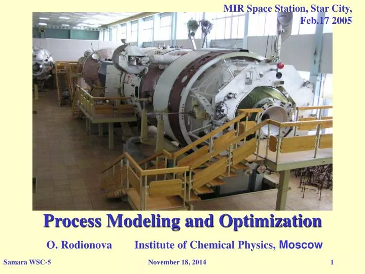
MIR Space Station, Star City, Feb.17 2005. Process Modeling and Optimization O. Rodionova Institute of Chemical Physics, Moscow. Based on Paper. Process control and optimization with simple interval calculation method Pomerantsev a , O. Rodionova a , and A. Höskuldsson b

E N D
MIR Space Station, Star City, Feb.17 2005 Process Modeling and OptimizationO. Rodionova Institute of Chemical Physics, Moscow Samara WSC-5
Based on Paper • Process control and optimization with simple interval calculation method • Pomerantseva, O. Rodionovaa, and A. Höskuldssonb • a Semenov Institute of Chemical Physics, Moscow, Russia • b Technical University of Denmark, Lyngby, Denmark in print Samara WSC-5
Outline • Introduction • Real-world example – description • Passive optimization • Sic- in brief • Active optimization • Conclusions Samara WSC-5
PAT – a gift for chemometrics(Process Analytical Technology) “MAN WITH THE GIFT” by Natar Ungalaq Guidance for Industry PAT — A Framework for Innovative Pharmaceutical Development, Manufacturing, and Quality Assurance Pharmaceutical CGMPs, September 2004 FDA = U.S. Department of Health and Human Services Food and Drug Administration Samara WSC-5
PAT Tools Multivariate tools for design, data acquisition and analysis Process analyzers Process control tools Continuous improvement and knowledge management tools (Guidance …) Samara WSC-5
Multivariate Statistical Process Control (MSPC) • MSPC Objective • To monitor the performance of the process • MSPC Concept • To study historical data representing good past process behavior • MSPC Method • Projection methods of Multivariate Data Analysis (PCA, PCR, PLS) • MSPC Approach • To plot multivariate score and control limits plots to monitor the process behavior Samara WSC-5
Multivariate Statistical Process Optimization (MSPO) • MSPO Objective • To optimize the performance of the process (product quality) • MSPO Concept • To study historical data representing good past process behavior • MSPO Method • Projection methods and Simple Interval Calculation (SIC) method • MSPO Approach • To plot predicted quality at each process stage Samara WSC-5
Real-world Example (strong drink production) Samara WSC-5
Technological Scheme. Multistage Process Samara WSC-5
Data Set Description X preprocessing Y preprocessing Samara WSC-5
Quality Data (Standardized Y Set) Samara WSC-5
Overall PLS Model Samara WSC-5
Passive Optimization in Practice Thinker by Rodin Samara WSC-5
Main Features • Objective • To predict future process output being in the middle of the process • Concept • To study historical data representing good past process behavior • Method • PLS and Simple Interval Prediction • Approach • Expanded Multivariate Process Modeling (E-MSPC) Samara WSC-5
Expanded Modeling. Example Samara WSC-5
Expanded PLS modeling Samara WSC-5
Simple Interval Calculations (SIC) in brief Triple Mobius by F. Brown Samara WSC-5
b V + V — SIC main steps Samara WSC-5
Definition 1.SIC-residual is defined as – This is a characteristic of bias v+ 2bh y–b br Definition 2.SIC-leverage is defined as – This is a normalized precision y v – y+b SIC-Residual and SIC-Leverage They characterize interactions between prediction and error intervals Samara WSC-5
RESULTS Initial Data Set {X,Y} Procedure Flow-Chart PLS/PCR model Fixed number of PCs SIC-modeling RESULTS yhat RMSEC RMSEP Samara WSC-5
SIC Prediction. All Test Samples Samara WSC-5
Expanded ModelingPLS + SIC Samara WSC-5
Expanded SIC modeling Samara WSC-5
Samples 2 & 3 Samara WSC-5
Samples 4 & 5 Samara WSC-5
? ? Prediction of y Passive Optimization. StageV PLS/SICprediction Samara WSC-5
The Necessity of Active Optimization • F. Yacoub, J.F. MacGregor Product optimization and control in the latent variable space of nonlinear PLS models. Chemom. Intell. Lab. Syst 70:63-74, 2004 • B.-H. Mevik, E. M. Færgestad, M. R. Ellekjær, T. Næs Using raw material measurements in robust process optimization Chemom. Intell. Lab. Syst 55:135-145, 2001 • Höskuldsson Causal and path modelling. Chemom. Intell. Lab. Syst., 58: 287-311, 2001 Samara WSC-5
Active Optimization in Practice “Let Us Beat Our Swords into Ploughshares” by Vuchetich’ Samara WSC-5
Dubious Result of Optimization Predicted Xopt variables are out of model! Samara WSC-5
Main Features • Objective • To find corrections for each process stage that improve the future process output (product quality) • Concept • Corrections are admissible if they are similar to ones that sometimes happened in the historical data in the similar situation • Method • PLS1, PLS2, SIC • Approach • Multivariate Statistical Process Optimization (MSPO) Samara WSC-5
PLS1 XY: (X,Z) y PLS2 XZ: X Z Intermediate Stage The Scheme of Three Data Block Modeling Samara WSC-5
Stage II XIIWR1,WR2 PLS1 Quality measureY Fixed variablesXfix Optimized Z Quality measureY PLS1 Model Y = X*a = Xfix b+ Z*c, where a=b+c Task For new (x,z) maximize(xtb+ztc) w.r.t. z, zLz Solution max (y) = Xfix b+ max (zt)*c, as all a > 0 (by g factor) Optimization Problem Stage I XIW1, W2, W3 ,S1, S2, S3 Samara WSC-5
Linear Optimization Linear function always reaches extremum at the border. So, the main problem of linear optimization is not to find a solution, but to restrict the area, where this solution should be found. Samara WSC-5
Lz Optimization restrictions I. All process and quality variables should be inside predefined control limits. |xi|1 and |yj|1 for every i,j II. Adjusted variables should not contradict process model For new (x,z) maximize(xtb+ztc) w.r.t. z, zLz Samara WSC-5
mh=0.83 sh=0.26 md=0.052 sd=0.031 How to define Lz ? PLS1 XY: X y Xtest l0=mh, l1=mh+sh, l2=mh+2sh, l3=mh+3sh, r0=md, r1=md+sd, r2=md+2sd, r3=md+3sd, Samara WSC-5
PLS2 XZ: X Z 0.075 0.025 z2 i -0.025 z1 i -0.075 Three optimization strategies Samara WSC-5
Strategy G1 Samara WSC-5
Sample 5 Normal Quality Insider (G3) Samara WSC-5
Sample 3 Normal Quality Abs. Outsider (G3) Samara WSC-5
Sample 4 Low Quality Outsider (G3) Samara WSC-5
Results of Optimization. Quality variable Samara WSC-5
Results of Optimization Samara WSC-5
Conclusions The presented optimization methods are based on the PLS block modeling as well as on the Simple Interval Calculation Application of the series of expanding PLS/SIC models helps to predict the effect of planned actions on the product quality, and thus enables passive quality optimization. For active optimization: (1) No improvement in quality obtained “inside” the model; (2) To yield a considerable improvement in y, the optimized variable values should be located in the boarder of the model; (3) It is obligatory to verify that optimized values do not contradict the process history. Samara WSC-5