Download
1 / 52
520 likes | 586 Views
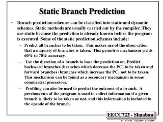
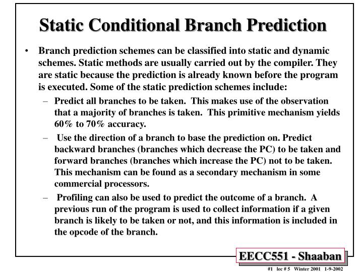
Static Conditional Branch Prediction.

E N D
Static Conditional Branch Prediction • Branch prediction schemes can be classified into static and dynamic schemes. Static methods are usually carried out by the compiler. They are static because the prediction is already known before the program is executed. Some of the static prediction schemes include: • Predict all branches to be taken. This makes use of the observation that a majority of branches is taken. This primitive mechanism yields 60% to 70% accuracy. • Use the direction of a branch to base the prediction on. Predict backward branches (branches which decrease the PC) to be taken and forward branches (branches which increase the PC) not to be taken. This mechanism can be found as a secondary mechanism in some commercial processors. • Profiling can also be used to predict the outcome of a branch. A previous run of the program is used to collect information if a given branch is likely to be taken or not, and this information is included in the opcode of the branch.
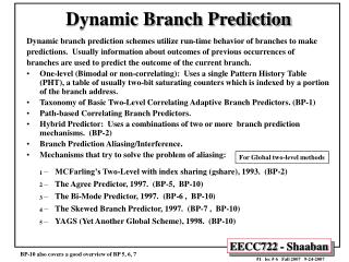
Dynamic Conditional Branch Prediction • Dynamic branch prediction schemes are different from static mechanisms because they use the run-time behavior of branches to make more accurate predictions than possible using static prediction. • Usually information about outcomes of previous occurrences of a given branch (branching history) is used to predict the outcome of the current occurrence. Some of the proposed dynamic branch prediction mechanisms include: • One-level or Bimodal: Uses a Branch History Table (BHT), a table of usually two-bit saturating counters which is indexed by a portion of the branch address (low bits of address). • Two-Level Adaptive Branch Prediction. • MCFarling’s Two-Level Prediction with index sharing (gshare). • Hybrid Predictor: Uses a combinations of two or more branch prediction mechanisms. • To reduce the stall cycles resulting from correctly predicted taken branches to zero cycles, a Branch Target Buffer (BTB) that includes the addresses of conditional branches that were taken along with their targets is added to the fetch stage.
Branch Target Buffer (BTB) • Effective branch prediction requires the target of the branch at an early pipeline stage. • One can use additional adders to calculate the target, as soon as the branch instruction is decoded. This would mean that one has to wait until the ID stage before the target of the branch can be fetched, taken branches would be fetched with a one-cycle penalty. • To avoid this problem one can use a Branch Target Buffer (BTB). A typical BTB is an associative memory where the addresses of branch instructions are stored together with their target addresses. • Some designs store n prediction bits as well, implementing a combined BTB and BHT. • Instructions are fetched from the target stored in the BTB in case the branch is predicted-taken. After the branch has been resolved the BTB is updated. If a branch is encountered for the first time a new entry is created once it is resolved. • Branch Target Instruction Cache (BTIC): A variation of BTB which caches the code of the branch target instruction instead of its address. This eliminates the need to fetch the target instruction from the instruction cache or from memory.
Hardware Dynamic Branch Prediction • Simplest method: • A branch prediction buffer or Branch History Table (BHT) indexed by low address bits of the branch instruction. • Each buffer location (or BHT entry) contains one bit indicating whether the branch was recently taken or not. • Always mispredicts in first and last loop iterations. • To improve prediction accuracy, two-bit prediction is used: • A prediction must miss twice before it is changed. • Two-bit prediction is a specific case of n-bit saturating counter incremented when the branch is taken and decremented otherwise. • Based on observations, the performance of two-bit BHT prediction is comparable to that of n-bit predictors.
One-Level Bimodal Branch Predictors • One-level or bimodal branch prediction uses only one level of branch history. • These mechanisms usually employ a table which is indexed by lower bits of the branch address. • The table entry consists of n history bits, which form an n-bit automaton. • Smith proposed such a scheme, known as the Smith algorithm, that uses a table of two-bit saturating counters. • One rarely finds the use of more than 3 history bits in the literature. • Two variations of this mechanism: • Decode History Table: Consists of directly mapped entries. • Branch History Table (BHT): Stores the branch address as a tag. It is associative and enables one to identify the branch instruction during IF by comparing the address of an instruction with the stored branch addresses in the table.
Decode History Table (DHT) N Low Bits of Table has 2N entries.
Basic Dynamic Two-Bit Branch Prediction: Two-bit Predictor State Transition Diagram
Prediction Accuracy of A 4096-Entry Basic Dynamic Two-Bit Branch Predictor
From The Analysis of Static Branch Prediction : DLX Performance Using Canceling Delay Branches
Prediction Accuracy of Basic Two-Bit Branch Predictors: 4096-entry buffer Vs. An Infinite Buffer Under SPEC89
Two-Level Adaptive Predictors • Two-level adaptive predictors were originally proposed by Yeh and Patt in 1991. • They use two levels of branch history. • The first level stored in a History Register (Table) (HRT), usually a k-bit shift register. • The data in this register is used to index the second level of history, the Pattern History Table (PHT). • Yeh and Patt later identified nine variations of this mechanism depending on how branch history and pattern history is kept: per address, globally or per set, plus they give a taxonomy.
Two-Level Adaptive Branch Predictors ( PHT ) Second Level First Level Or Table ( HRT )
Taxonomy of Two-level Adaptive Branch Prediction Mechanisms Second level First level
Variations of global history Two-Level Adaptive Branch Prediction.
Variations of per-address historyTwo-Level Adaptive Branch Prediction
Variations of per-set history Two-Level Adaptive Branch Prediction
Hardware cost of Two-level Adaptive Prediction Mechanisms • Neglecting logic cost and assuming 2-bit of pattern history for each entry. The parameters are as follows: • k is the length of the history registers, • b is the number of branches, • p is the number of sets of branches in the PHT, • s is the number of sets of branches in HRT.
GAp Predictor • The branch history (first level) is kept globally in a history register, and is used to select one of the pattern history tables (second level) which are kept per branch address.
Correlating Branches Recent branches are possibly correlated: The behavior of recently executed branches affects prediction of current branch. Example: Branch B3 is correlated with branches B1, B2. If B1, B2 are both not taken, then B3 will be taken. Using only the behavior of one branch cannot detect this behavior. SUBI R3, R1, #2 BENZ R3, L1 ; b1 (aa!=2) ADD R1, R0, R0 ; aa==0 L1: SUBI R3, R1, #2 BNEZ R3, L2 ; b2 (bb!=2) ADD R2, R0, R0 ; bb==0 L2 SUB R3, R1, R2 ; R3=aa-bb BEQZ R3, L3 ; b3 (aa==bb) B1 if (aa==2) aa=0; B2 if (bb==2) bb=0; B3 if (aa!==bb){
Correlating Two-Level Dynamic GAp Branch Predictors • Improve branch prediction by looking not only at the history of the branch in question but also at that of other branches: • Record the pattern of the m most recently executed branches as taken or not taken. • Use that pattern to select the proper branch history table. • In general, the notation: (m,n) GAp predictor means: • Record last m branches to select between 2m history tables. • Each table uses n-bit counters (each table entry has n bits). • Basic two-bit single-level Bimodal BHT is then a (0,2) predictor.
if (d==0) d=1; if (d==1) BNEZ R1, L1 ; branch b1 (d!=0) ADDI R1, R0, #1 ; d==0, so d=1 L1: SUBI R3, R1, #1 BNEZ R3, L2 ; branch b2 (d!=1) . . . L2: Dynamic Branch Prediction: Example
if (d==0) d=1; if (d==1) Dynamic Branch Prediction: Example (continued) BNEZ R1, L1 ; branch b1 (d!=0) ADDI R1, R0, #1 ; d==0, so d=1 L1: SUBI R3, R1, #1 BNEZ R3, L2 ; branch b2 (d!=1) . . . L2:
Organization of A Correlating Two-level GAp (2,2) Branch Predictor
Prediction Accuracy of Two-Bit Dynamic Predictors Under SPEC89 Basic Basic Correlating Two-level GAp
MCFarling's gshare Predictor • McFarling notes that using global history information might be less efficient than simply using the address of the branch instruction, especially for small predictors. • He suggests using both global history and branch address by hashing them together. He proposes using the XOR of global branch history and branch address since he expects that this value has more information than either one of its components. The result is that this mechanism outperforms a GAp scheme by a small margin. • This mechanism seems to use substantially less hardware, since both branch and pattern history are kept globally. • The hardware cost for k history bits is k + 2 x 2k , neglecting costs for logic.
gshare Predictor Branch and pattern history are kept globally. History and branch address are XORed and the result is used to index the pattern history table.
Hybrid or Combined Predictors • Hybrid predictors are simply combinations of other branch prediction mechanisms. • This approach takes into account that different mechanisms may perform best for different branch scenarios. • McFarling presented a number of different combinations of two branch prediction mechanisms. • He proposed to use an additional 2-bit counter array which serves to select the appropriate predictor. • One predictor is chosen for the higher two counts, the second one for the lower two counts. • If the first predictor is wrong and the second one is right the counter is decremented, if the first one is right and the second one is wrong, the counter is incremented. No changes are carried out if both predictors are correct or wrong.
MCFarling’s Combined Predictor Structure The combined predictor contains an additional counter array with 2-bit up/down saturating counters. Which serves to select the best predictor to use. Each counter keeps track of which predictor is more accurate for the branches that share that counter. Specifically, using the notation P1c and P2c to denote whether predictors P1 and P2 are correct respectively, the counter is incremented or decremented by P1c-P2c as shown below.
Processor Branch Prediction Comparison Processor Released Accuracy Prediction Mechanism Cyrix 6x86 early '96 ca. 85% BHT associated with BTB Cyrix 6x86MX May '97 ca. 90% BHT associated with BTB AMD K5 mid '94 80% BHT associated with I-cache AMD K6 early '97 95% 2-level adaptive associated with BTIC and ALU Intel Pentium late '93 78% BHT associated with BTB Intel P6 mid '96 90% 2 level adaptive with BTB PowerPC750 mid '97 90% BHT associated with BTIC MC68060 mid '94 90% BHT associated with BTIC DEC Alpha early '97 95% 2-level adaptive associated with I-cache HP PA8000 early '96 80% BHT associated with BTB SUN UltraSparc mid '95 88%int BHT associated with I-cache 94%FP
The Cyrix 6x86/6x86MX • Both use a single-level 2-bit Smith algorithm BHT associated with BTB. • BTB (512-entry for 6x86MX and 256-entry for 6x86) and the BHT (1024-entry for 6x86MX). • The Branch Target Buffer is organized 4-way set-associative where each set contains the branch address, the branch target addresses for taken and not-taken and 2-bit branch history information. • Unconditional branches are handled during the fetch stage by either fetching the target address in case of a BTB hit or continuing sequentially in case of a BTB miss. • For conditional branch instructions that hit in the BTB the target address according to the history information is fetched immediately. Branch instructions that do not hit in the BTB are predicted as not taken and instruction fetching continues with the next sequential instruction. • Whether the branch is resolved in the EX or in the WB stage determines the misprediction penalty (4 cycles for the EX and 5 cycles for the WB stage). • Both the predicted and the unpredicted path are fetched. avoiding additional cycles for cache access when a misprediction occurs. • Return addresses for subroutines are cached in an eight-entry return stack on which they are pushed during CALL and popped during the corresponding RET.
Intel Pentium • Similar to 6x86, it uses a single-level 2-bit Smith algorithm BHT associated with a four way associative BTB which contains the branch history information. • However Pentium does not fetch non-predicted targets and does not employ a return stack. • It also does not allow multiple branches to be in flight at the same time. • However, due to the shorter Pentium pipeline (compared with 6x86) the misprediction penalty is only three or four cycles, depending on what pipeline the branch takes.
Intel P6,II,III • Like Pentium, the P6 uses a BTB that retains both branch history information and the predicted target of the branch. However the BTB of P6 has 512 entries reducing BTB misses. Since the • The average misprediction penalty is 15 cycles. Misses in the BTB cause a significant 7 cycle penalty if the branch is backward • To improve prediction accuracy a two-level branch history algorithm is used. • Although the P6 has a fairly satisfactory accuracy of about 90%, the enormous misprediction penalty should lead to reduced performance. Assuming a branch every 5 instructions and 10% mispredicted branches with 15 cycles per misprediction the overall penalty resulting from mispredicted branches is 0.3 cycles per instruction. This number may be slightly lower since BTB misses take only seven cycles.
AMD K5 • The branch history information is included in the instruction cache together with the location of the target instruction within the cache. This approach is very inexpensive since no BTB is used and only the location of the target within the instruction cache rather than the full address is stored. • This approach allows AMD to keep 1024 branches predicted. However, it could happen that the target line which is referred to in a different line of the cache has already been overwritten, or that the target address is computed and has changed between two calls of a particular branch. • To avoid wrong target instructions to be fetched a branch unit address comparison logic is employed. • The performance is comparable with that of Intel Pentium.
AMD K5 Instruction Cache Integrated Branch Prediction Mechanism
AMD K6 • Uses a two-level adaptive branch history algorithm implemented in a BHT with 8192 entries (16 times the size of the P6). • However, the size of the BHT prevents AMD from using a BTB or even storing branch target address information in the instruction cache. Instead, the branch target addresses are calculated on-the-fly using ALUs during the decode stage. The adders calculate all possible target addresses before the instruction are fully decoded and the processor chooses which addresses are valid. • A small branch target cache (BTC) is implemented to avoid a one cycle fetch penalty when a branch is predicted taken. • The BTC supplies the first 16 bytes of instructions directly to the instruction buffer. • Like the Cyrix 6x86 the K6 employs a return address stack for subroutines. • The K6 is able to support up to 7 outstanding branches. • With a prediction accuracy of more than 95% the K6 outperforms all other current microprocessors (except the DEC Alpha).
Motorola PowerPC 750 • A dynamic branch prediction algorithm is combined with static branch prediction which enables or disables the dynamic prediction mode and predicts the outcome of branches when the dynamic mode is disabled. • Uses a single-level Smith algorithm 512-entry BHT and a 64-entry Branch Target Instruction Cache (BTIC), which contains the most recently used branch target instructions, typically in pairs. When an instruction fetch does not hit in the BTIC the branch target address is calculated by adders. • The return address for subroutine calls is also calculated and stored in user-controlled special purpose registers. • The PowerPC 750 supports up to two branches, although instructions from the second predicted instruction stream can only be fetched but not dispatched.
The HP PA 8000 • The HA PA 8000 uses static branch prediction combined with dynamic branch prediction. • The static predictor can turn the dynamic predictor on and off on a page-by-page basis. It usually predicts forward conditional branches as not taken and backward conditional branches as taken. • It also allows compilers to use profile based optimization and heuristic methods to communicate branch probabilities to the hardware. • Dynamic bench prediction is implemented by a 256-entry BHT where each entry is a three bit shift register which records the outcome of the last three branches instead of saturated up and down counters. The outcome of a branch (taken or not taken) is shifted in the register as the branch instruction retires. • To avoid a taken branch penalty of one cycle the PA 8000 is equipped with a Branch Target Address Cache (BTAC) which has 32 entries.
The SUN UltraSparc • Uses a single-level BHT Smith algorithm. • It employs a static prediction which is used to initialize the state machine (saturated up and down counters). • However, the UltraSparc maintains a large number of branch history entries (up to 2048 or every other line of the I-cache). • To predict branch target addresses a branch following mechanism is implemented in the instruction cache. The branch following mechanism also allows several levels of speculative execution. • The overall performance of UltraSparc is 94% for FP applications and 88% for integer applications.
The Compaq Alpha 21264 • The Alpha 21264 uses a two-level adaptive hybrid method combining two algorithms (a global history and a per-branch history scheme) and chooses the best according to the type of branch instruction encountered • The prediction table is associated with the lines of the instruction cache. An I-cache line contains 4 instructions along with a next line and a set predictor. • If an I-cache line is fetched that contains a branch the next line will be fetched according to the line and set predictor. For lines containing no branches or unpredicted branches the next line predictor point simply to the next sequential cache line. • This algorithm results in zero delay for correct predicted branches but wastes I-cache slots if the branch instruction is not in the last slot of the cache line or the target instruction is not in the first slot. • The misprediction penalty for the alpha is 11 cycles on average and not less than 7 cycles. • The resulting prediction accuracy is about 95% very good. • Supports up to 6 branches in flight and employs a 32-entry return address stack for subroutines.