Download
1 / 29
290 likes | 376 Views
Array types:. numeric character logical cell structure function handle Java. MAT rix LAB oratory. The name says it all: Matlab is designed for work with matrices A matrix is an arrangement of numbers in a rectangular pattern An m by n matrix has m rows n columns

E N D
Array types: numeric character logical cell structure function handle Java
MATrixLABoratory • The name says it all: Matlab is designed for work with matrices • A matrix is an arrangement of numbers in a rectangular pattern • An m by n matrix has • m rows • n columns • mn elements of (floating point) numbers
A = magic(4) • Each row adds to 34 • Each colum adds to 34 • Each diagonal adds to 34 • A(1,1) element in upper left corner • A(i,j) element in i-th row and j-th column • Note: Numbering starts with 1 (and not with 0, as some other programming languages do) • Starting with 1 is used frequently in mathematics • Starting with 0 is more natural for implementation in a computer
Creating matrices • B=[16,2,3,13;5,11,10,8;9,7,6,12;4,14,15,1] • Values are given as integers, but stored as floating point numbers • Elements of a row are separated by a space or a comma • Rows are separated by semicolon • Number of elements have to be the same in each row
Special Matrices • Row vector (1 by n matrix) • a = [ 1 , 2 , 3 , 4 ] • Column vector (m by 1 matrix) • b = [ 1 ; 2 ; 3 ; 4 ] • Transpose of a matrix - Interchange rows with columns • c = a' • c is now the same as b
Referencing elements of an array (matrix) • A= magic(4) 4 by 4 matrix • A(2,3) specific element in row 2 • A(2, 2:4) row vector from row 2 of A with elements 2 to 4 • A(1:3,3) column vector from column 3 of A with elements 1 to 3 • A(1:2:3,4) column vector from column 4 of A with elements 1 and 3 • A(:,3) entire column 3 of A • A(1:2, 2:3) submatrix of A
Indexing • via a specific value • range of values created via • start:inc:stop • default for inc is 1 • if value for stop is not known can use keyword 'end' instead, which will refer to largest value for that index • : refers to all defined values for that index
Array operations • Matlab allows use of index notation on the right and also on the left hand side of an assignment statement • Most other programming languages are much more restrictive • in C++ A[2][3] references an element • but A[2] gives the address of row 2, which can not be changed • Since Matlab extends arrays automatically need to watch out for referencing undefined elements: • A=magic(4) ; A(2,3:5)=[21,47,45] • is ok in Matlab
Functions operating on vectors • v vector (row or column) • max(v) returns largest element in v • min(v) returns smallest element in v • find(v) returns indices of nonzero elements in v • sort(v) returns vector sorted in ascending order • sum(v) returns sum of the elements in v • length(v) • size(v) gives dimensions of the array v, i.e. • 1 length(v) for a row vector • or • length(v) 1 for a column vector
Representation of arrays in Matlab • A = [2, 6, 9; 4, 2, 8; 3, 5, 1] • A = • 2 6 9 • 4 2 8 • 3 5 1 • is actually stored in memory as the sequence • 2, 4, 3, 6, 2, 5, 9, 8, 1 • that is in column major form, as done by Fortran • Most other programming languages use row major form, i.e. order in which elements are entered
Functions applied to matrices • A m , n matrix • max(A), min(A), sort(A), sum(A) return row vectors with operation performed on each column • find(v) returns linear indices of nonzero elements in A • linear index of element A(i,j) is (j-1)m + i • [u,v,w] = find(A) gives a more useful result • u vector for row indices • v vector for column indices • w vector with non-zero elements • length(A) returns maximum of m and n • size(A) returns dimension of A, that is m n
Other methods for creating a vector (one dimensional array) • x = [ -10 : 3 : 10 ] • same as x = [-10 , -7, -4, -1, 2, 5, 8 ] • y = [ 10 : -3 : -10] • same as y =[ 10, 7, 4, 1, -2, -5, -8] • z = [ 0 : 10 ] • default increment is 1 • linspace( x1, x2, n ) • n number of points (values) between x1 and x2 inclusive endpoints x1 and x2 • xx = linspace( 5, 8, 10 ) • same as xx = [5 : 0.3333333333333333 : 10] • logspace( a, b, n) • n number of points between 10a and 10b includes endpoints • xlog = logspace( 1, 2, 10 )
logspaceprogram that does the same a = 1 b = 2 n = 10 inc = 10^((b – a ) / n ) myxlog(1) = 10^a for k = 2 : n myxlog(k) = myxlog(k-1) * inc end
Remarks • If the program is converted to a script do not call it logspace.m • otherwise original command is no longer available. • removing file logspace.m from directory causes also problems since Matlab maintains history of functions used • information kept in tool_path_cache • clear myxlog • should be at the beginning of the script • old values from a previous use of mylogspace will still be visible
Remarks • Scalars are arrays of length 1 • k = 1 • k(1) is defined but not k(2) • Arrays (vectors and matrices) can be extended by assigning an array element outside the current bounds • any missing elements will be set to 0 • k(4) = 23 • the array k has now elements [1, 0, 0, 23]
Remarks • A = [1,2,3 ; 4,5,6] • A(1,5) = 23 • gives new 3 by 5 matrix • 1 2 3 0 23 • 4 5 6 0 0 • Most programming languages do not allow the extension of an existing array. For these languages • Size of the array has to declared at the beginning • Exceeding the bounds of an array causes a run time error (not a compile time error) • Some programming languages i.e. Java will detect this type of error and terminate the run with an error message • Other programming languages i.e. C and C++ will overwrite an adjacent storage location with unpredictable results
Multi dimensional arrays • A(3,2,4) element of a three dimensional array • Note how Matlab fills in missing elements and display new array • Information about workspace variables is updated automatically • Creating multi dimensional arrays • by assigning individual elements • or with notation cat(n, A, B, C,…) • where A, B, C,…all are arrays of the same size • n the dimension where the matrices are catenated • example cat(1,A,B) cat(2,A,B) cat(3,A,B)
Use of vectors in geometry • Common operations • vector addition: u+v • vector subtraction: u-v • multiplication with a scalar r: ru • length of a vector |u| • dot product: uv =|u| |v| cos() • with angle between u and v • dot product multiplies elements of u and v pairwise and adds them together • uu = |u|2
Use of matrices in geometry • defines linear transformation y = A x • x column vector of length n • y column vector of length m • A matrix of size m by n • for the multiplication A x take each row of A and form the dot product with x • Note the requirement that the number of elements in a row of A has to be the same as the number of elements in the column of x
Operations on arrays in Matlab • Matlab provides many different operations for arrays (vectors, matrices, multi dimensional arrays) • Some of the operations have a geometric interpretation, others do not • If there are certain requirements for performing on operation it comes from conforming to the geometric interpretation of the operation • See course on 'Matrix Methods'
Element by element operations for arrays of the same size • Scalar b added to array A: A + b • Scalar b subtracted from array A: A – b • Addition of two arrays: A + B • Subtraction of two arrays: A – B • Multiplication of two arrays: A . B • Right division of two arrays: A ./ B • Left division of two arrays: A .\ B • Array exponentiation: A .^ B
Remarks • The last 4 operations have no geometric interpretation • The first two operations are mathematically incorrect, b should be vector with all of its elements set to b • Matlab allows standard functions to operate on each element of an array and produces an array of the same size • For example sqrt(A) or cos(A), again the resulting matrices do not conform to the mathematical definition of sqrt(A) or cos(A)
Array operations in Matlab • Geometric interpretation not needed, when evaluating functions at many points • t=[ 0 : 0.003 : 0.5 ] ; • array t(1)=0 to t(167)=0.498 • y = exp(-8 * t ) .* sin(9.7 * t +pi/2) ; • exp(-8*t) evaluates to an array of length 167 • sin(9.7*t+pi/2) evaluates to an array • in order to multiply individual terms of the two arrays need to use .*
General Comments for Plotting • Use … in order to continue a statement on next line • Number of points for plotting should be enough to give a smooth graph • but not so many so that it would take too long to evaluate functions and exceed available memory • labels for each axis should give dimension
Current and power dissipation in resistors • current: I • volt: V • resistance: R • Ohm's law I = V/R • Power dissipation Watts: I*V=I2/R • in Matlab given arrays for V and R • need to use .^ and ./ • watts = V.^2./R • In order to make statement clearer use parentheses • watts = (V.^2) ./ R
Solving equations by graphical means • Given L = 70 find approximate value for x • [x,y]=ginput(n) • graphical input from mouse and cursor • option to plot, allows fixing of n coordinate lines with the click of the mouse