Download
1 / 11
120 likes | 225 Views
The use of curvature in potential-field interpretation Exploration Geophysics , 2007, 38 , 111–119 Phillips, Hansen, & Blakely

E N D
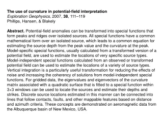
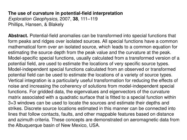
The use of curvature in potential-field interpretation Exploration Geophysics, 2007, 38, 111–119 Phillips, Hansen, & Blakely Abstract. Potential-field anomalies can be transformed into special functions that form peaks and ridges over isolated sources. All special functions have a common mathematical form over an isolated source, which leads to a common equation for estimating the source depth from the peak value and the curvature at the peak. Model-specific special functions, usually calculated from a transformed version of a potential field, are used to estimate the locations of very specific source types. Model-independent special functions calculated from an observed or transformed potential field can be used to estimate the locations of a variety of source types. Vertical integration is a particularly useful transformation for reducing the effects of noise and increasing the coherency of solutions from model-independent special functions. For gridded data, the eigenvalues and eigenvectors of the curvature matrix associated with a quadratic surface that is fitted to a special function within 3×3 windows can be used to locate the sources and estimate their depths and strikes. Discrete source locations estimated in this manner can be connected into lines that follow contacts, faults, and other mappable features based on distance and azimuth criteria. These concepts are demonstrated on aeromagnetic data from the Albuquerque basin of New Mexico, USA.
The use of curvature in potential-field interpretation,Exploration Geophysics, 2007, 38, 111–119. Phillips, Hansen, & Blakely.
The use of curvature in potential-field interpretation,Exploration Geophysics, 2007, 38, 111–119. Phillips, Hansen, & Blakely.
The use of curvature in potential-field interpretation,Exploration Geophysics, 2007, 38, 111–119. Phillips, Hansen, & Blakely.
The use of curvature in potential-field interpretation,Exploration Geophysics, 2007, 38, 111–119. Phillips, Hansen, & Blakely.
The use of curvature in potential-field interpretation,Exploration Geophysics, 2007, 38, 111–119. Phillips, Hansen, & Blakely.
The use of curvature in potential-field interpretation,Exploration Geophysics, 2007, 38, 111–119. Phillips, Hansen, & Blakely.
The use of curvature in potential-field interpretation,Exploration Geophysics, 2007, 38, 111–119. Phillips, Hansen, & Blakely.
From: The use of curvature in potential-field interpretation Exploration Geophysics, 2007, 38, 111–119. Phillips, Hansen & Blakely. Comparison of results A composite view of the estimated contact and fault locations (Figure 4d) shows how the total gradient solutions from the half vertical integral of the TMI (in green) and the local wavenumber solutions from the first vertical integral of the TMI (in blue) typically plot close together. The horizontal gradient solutions from the reduced-to-pole field (in red) tend to be the most coherent and most easily interpreted. They are typically offset from the blue and green solutions, most likely due to non-vertical dips on the faults and contacts. Model studies (Phillips, 2000) indicate that, for magnetisations collinear with the inducing field, the offset of the HGM solutions should be in the down-dip direction.
From Phillips’: USGS_SFDEPTH GX – as implemented in Oasis Montaj The following model-specific special functions are supported : Assumed_Source_Type SI Transform Model-Specific_Special_Function Vertical_Magnetic_Contact 0 RTP HGM of RTP magnetic field Vertical Magnetic Sheet 1 RTP ABS of RTP magnetic field Horizontal Magnetic Sheet 1 RTP+VI HGM of VI of RTP magnetic field Horizontal Magnetic Line 2 RTP+VI ABS of VI of RTP magnetic field Vertical Magnetic Line 2 RTP+VI ABS of VI of RTP magnetic field Magnetic Dipole 3 RTP+VI ABS of VI of RTP magnetic field Vertical Density Contact -1 VD HGM of VD of gravity field Vertical Density Sheet 0 VD ABS of VD of gravity field Horizontal Density Sheet 0 None HGM of gravity field Horizontal Density Line 1 None ABS of gravity field Vertical Density Line 1 None ABS of gravity field Point Mass 2 None ABS of gravity field Model-independent special functions include the Total Gradient (TG) and the Local Wavenumber (LW). These are calculated directly from the potential field or from a vertical integral (VI) of the potential field. The total gradient requires that a structural index (SI) be assumed for the source.