Integer transform
500 likes | 762 Views
Integer transform. Wen - Chih Hong E-mail: pippo.cm93@nctu.edu.tw Graduate Institute of Communication Engineering National Taiwan University, Taipei, Taiwan, ROC. 1. Outline. 1. Introduction what is integer why integer 2. General method

Integer transform
E N D
Presentation Transcript
Integer transform Wen - Chih Hong E-mail: pippo.cm93@nctu.edu.tw Graduate Institute of Communication Engineering National Taiwan University, Taipei, Taiwan, ROC 1
Outline 1. Introduction what is integer why integer 2. General method 3. Matrix factorization 4. Modified matrix factorization 5. Conclusions 6. Reference 2
Introduce : what is integer transform 1. all entries are integer i.e. -5,-3,0,2,… 2.all entries are sum of power of 2 i.e. 3
Introduction : Why integer transform We can use the fix-point multiplication operation to replace floating-point one to implement it 4
Introduction : The constraints of approximated integer transform 1. if A(m,n1)=τA(m,n2) , τ=1,-1,j,-j then B(m,n1)=τB(m,n2) 2. if Re(A(m,n1)) ≥ Re(A(m,n2)) Im(A(m,n1)) ≥ Im(A(m,n2)) then Re(B(m,n1)) ≥ Re(B(m,n2)) Im(B(m,n1)) ≥ Im(B(m,n2)) 5
Introduction :The constraints of Approximated integer transform 3. if sgn(Re(A(m,n1)))=sgn((Re(A(m,n1))) then sgn(Re(B(m,n1)))=sgn((Re(B(m,n1))) 4. (*) 6
Introduction : algorithms We have three algorithms to approximate non-integer transform 1. General method 2. Matrix factorization 3. Modified matrix factorization 7
General method 1. Forming the prototype matrix 2. Constraints for Orthogonality (Equality Constraints) 3. Constraints for Inequality (Inequality Constraints) 4. Assign the values 8
Appendix - Principle of Dyadic symmetry(1/2) Definition: a vector [a0,a1,…,am-1] m=2^n we say it has the ith dyadic symmetry i.i.f. aj=s.a i j where i,j in the range [0,m-1] s= 1 when symmetry is even s=-1 when symmetry is odd 9
Appendix - Principle of Dyadic symmetry (2/2) For a vector of eight elements, there are seven possible dyadic symmetries. 10
General method : Generation of the order-8 ICTs(1/8) Take 8-order discrete cosine transform for example for i =0 for i =1~7 where j=0,1,…,6,7 (1) 11
General method : Generation of the order-8 ICTs(2/8) 0.3536 0.3536 0.3536 0.3536 0.3536 0.3536 0.3536 0.3536 0.4904 0.4157 0.2778 0.0975 -0.0975 -0.2778 -0.4157 -0.4904 0.4619 0.1913 -0.1913 -0.4619 -0.4619 -0.1913 0.1913 0.4619 0.4157 -0.0975 -0.4904 -0.2778 0.2778 0.4904 0.0975 -0.4157 0.3536 -0.3536 -0.3536 0.3536 0.3536 -0.3536 -0.3536 0.3536 0.2778 -0.4904 0.0975 0.4157 -0.4157 -0.0975 0.4904 -0.2778 0.1913 -0.4619 0.4619 -0.1913 -0.1913 0.4619 -0.4619 0.1913 0.0975 -0.2778 0.4157 -0.4904 0.4904 -0.4157 0.2778 -0.0975 Let T=kJ, k is diagonal matrix 12
General method : Generation of the order-8 ICTs(3/8) 1. Forming the prototype 13
General method : Generation of the order-8 ICTs(4/8) 2. Constraints for Orthogonality Sth dyadic symmetry type in basis vector Ji 14
General method : Generation of the order-8 ICTs(5/8) 2. Constraints for Orthogonality (i) Totally C(8,2)=28 equations must be satisfied (ii) Using principle of dyadic symmetry*, we can reduce 28 to 1 equation: a.b=a.c + b.d + c.d (2) 15
General method : Generation of the order-8 ICTs (6/8) 3. Constraints for Inequality the equation in page.8 imply a ≥ b ≥ c ≥ d ,and e ≥ f (3) 16
General method : Generation of the order-8 ICTs(7/8) 4. Assign the values : use computer to find all possible values (of course the values must be integer) 17
General method : Generation of the order-8 ICTs(8/8) Some example of (a, b, c, d, e, f): (3,2,1,1,3,1) ,(5,3,2,1,3,1),… infinity set solutions we need to define a tool to recognize which one is better 18
General method : Performance(1/2) In the transform coding of pictures Efficiency: (5) where 19
General method : Performance(2/2) The twelve order-8 ICTs that have the highest transform efficiencies for p equal 0.9 and a less than or equal to 255 20
General method : Disadvantage of general method • Too much unknowns. • need to satisfy a lot of equations ,C(n,2). • It has no reversibility. A’≈A , (A^-1)’≈(A^-1), but (A’)^-1≠ (A^-1)’ 21
Matrix Factorization Reversible integer mapping is essential for lossless source coding by transformation. General method can not solve the problem of reversibility 22
Matrix Factorization :algorithm(1/9) Goal : 1. Suppose A , and det(A) ≠ 0 (6) 23
Matrix Factorization :algorithm(2/9) 2. There must exist a permutation matrix for row interchanges s.t. (7) and 24
Matrix Factorization :algorithm(3/9) 3. There must exist a number s.t. then we get and a product (8) 25
Matrix Factorization :algorithm(4/9) 4. Multiplying an elementary Gauss matrix (9) 26
Matrix Factorization :algorithm(5/9) 5. Continuing in this way for k=1,2,…,N-1. defines the row interchanges among the through the rows to guarantee then we get where (10) 27
Matrix Factorization :algorithm(6/9) where (11) 28
Matrix Factorization :algorithm(7/9) 6. Multiplying all the SERMs ( ) together (12) 29
Matrix Factorization :algorithm(8/9) 7. (13) where 30
Matrix Factorization :algorithm (9/9) 8. we obtain or 9. Theorem (14) i.i.f. det(LU) is integer. 31
Matrix Factorization :Advantage if det(A) is integer then It is easy to derive the inverse of A 32
Modified matrix factorization:algorithm(1/6) If A is a NxN reversible transform 1. First, scale A by a constant , where such that : (15) 33
Modified matrix factorization:algorithm(2/6) 2. Do permutation and sign-changing operations for : , :arbitrary permutation matrix , :diagonal matrix (16) 34
Modified matrix factorization:algorithm(3/6) 3. Do triangular matrix decomposition. First, we find such that has the following form: (17) where 35
Modified matrix factorization:algorithm(4/6) 4. : Note that is also an upper-triangular matrix. (18) 36
Modified matrix factorization:algorithm(5/6) 5. Decompose into and . (19) where , From (8)(9)(10) we decompose ,then, 37
Modified matrix factorization:algorithm(6/6) 6. Approximates , , and by binary valued matrices , , and : 38
Modified matrix factorization:the process of forward transform Step 1: Step 2: for 39
Modified matrix factorization:the process of forward transform Step 3: for Step 4: when 40
Modified matrix factorization:the process of forward transform Step 5: 41
Modified matrix factorization:Accuracy analysis Preliminaries 1. where 2. is a random variable and uniformly distribute in [ , ] 3. and 42
Modified matrix factorization:Accuracy analysis The process in step (2)-(4) can be rewritten as: 43
Modified matrix factorization:Accuracy analysis If y=Gx=σAx then the difference between z, y is: (20) if b is very large in page.39 44
Modified matrix factorization:Accuracy analysis Using (20) to estimate the normalized root mean square error (NRMSE) and use it to measure the accuracy: 45
Modified matrix factorization:Accuracy analysis Notice (20) ,we find the NRMSE which is dominated by and . So we let the entries of T2 and T3 as small as possible . That why we multiply P, D, and Q to G. 46
Modified matrix factorization:Advantages Compare to matrix factorization : 1. simpler and faster way to derive the integer transform 2. Easier to design 3. Higher accuracy 48
Conclusions If a transform A ,which det(A) is an integer factor, we can convert it into integer transform. Integer transform is easy to implement, but is less accuracy than non-integer transform. It is a trade-off. 49
Reference 1. W.-K. Cham, PhD “Development of integer cosine transforms by the principle of dyadic symmetry” 2. W. K. Cham and Y. T. Chan” An Order-16 Integer Cosine Transform” 3. Pengwei Hao and Qingyun Shi “Matrix Factorizations for Reversible Integer Mapping” 4. Soo-Chang Peiand Jian-Jiun Ding” The Integer Transforms Analogous to Discrete Trigonometric Transforms” 5. Soo-Chang Pei and Jian-Jiun Ding” Improved Reversible Integer Transform” 50