Download
1 / 45
450 likes | 554 Views
Hash Table. 황승원 Fall 2010 CSE, POSTECH. Dictionaries. Collection of pairs. (key, element) Pairs have different keys. e.g., gradebook, phone book, e-dictionary Operations. get(theKey) put(theKey, theElement) remove(theKey)

E N D
Hash Table 황승원 Fall 2010 CSE, POSTECH
Dictionaries • Collection of pairs. • (key, element) • Pairs have different keys. e.g., gradebook, phone book, e-dictionary • Operations. • get(theKey) • put(theKey, theElement) • remove(theKey) • Array is an ideal special case where key (= “index” of array) is (1) consecutive (2) distinct integers
Application • Collection of student records in this class. • (key, element) = (student name, linear list of assignment and exam scores) • All keys are distinct. • Get the element whose key is John Adams. • Update the element whose key is Diana Ross. • put() implemented as update when there is already a pair with the given key. • remove() followed by put().
Dictionary With Duplicates • Keys are not required to be distinct. • Word dictionary. • Pairs are of the form (word, meaning). • May have two or more entries for the same word. • (bolt, a threaded pin) • (bolt, a crash of thunder) • (bolt, to shoot forth suddenly) • (bolt, a gulp) • (bolt, a standard roll of cloth) • etc.
Represent As A Linear List • L = (e0, e1, e2, e3, …, en-1) • Each ei is a pair (key, element). • 5-pair dictionary D = (a, b, c, d, e). • a = (aKey, aElement), b = (bKey, bElement), etc. • Array or linked representation.
a b c d e Array Representation • get(theKey) • O(size) time • put(theKey, theElement) • O(size) time to verify duplicate, O(1) to add at right end. • remove(theKey) • O(size) time.
A B C D E Sorted Array • elements are in ascending order of key. • get(theKey) • O(logsize) time • put(theKey, theElement) • O(logsize) time to verify duplicate, O(size) to add. • remove(theKey) • O(size) time (to rearrange)
firstNode null a b c d e Unsorted Chain • get(theKey) • O(size) time • put(theKey, theElement) • O(size) time to verify duplicate, O(1) to add at left end. • remove(theKey) • O(size) time.
firstNode null A B C D E Sorted Chain • Elements are in ascending order of Key. • get(theKey) • O(size) time • put(theKey, theElement) • O(size) time
firstNode null A B C D E Sorted Chain • remove(theKey) • O(size) time
Skip Lists • Idea: What if we have pointers pointing the half (or ¼, 1/8, …) We can simulate binary search • Worst-case time for get, put, and remove is O(size). • Expected time is O(log size).
Hash Tables • Worst-case time for get, put, and remove is O(size). • Expected time is O(1) Consider this whenever you need super-fast lookups
Ideal Hashing • Uses a 1D array (or table) table[0:b-1]. • Each position of this array is a bucket. • A bucket can normally hold only one dictionary pair. • Uses a hash function f thatconverts each key k into an index in the range [0, b-1]. • f(k) is the home bucket for key k. • Every dictionary pair (key, element) is stored in its home bucket table[f[key]].
[0] [1] [2] [3] [4] [5] [6] [7] Ideal Hashing Example • Pairs are: (22,a),(33,c),(3,d),(73,e),(85,f). • Hash table is table[0:7], b = 8. • Hash function is key/11 • Pairs are stored in table as below: (3,d) (22,a) (33,c) (73,e) (85,f) • get,put, andremove takeO(1)time.
[0] [1] [2] [3] [4] [5] [6] [7] What Can Go Wrong? • Where does (26,g) go? • Keys that have the same home bucket are synonyms. • 22 and 26 are synonyms with respect to the hash function that is in use. • The home bucket for (26,g) is already occupied.Collision!!!!!!! (3,d) (22,a) (33,c) (73,e) (85,f)
(3,d) (22,a) (33,c) (73,e) (85,f) What Can Go Wrong? • A collision occurs when the home bucket for a new pair is occupied by a pair with a different key. • An overflow occurs when there is no space in the home bucket for the new pair. • When a bucket can hold only one pair, collisions and overflows occur together. • Need a method to handle overflows.
Hash Table Issues • Choice of hash function. • Overflow handling method. • Size (number of buckets) of hash table.
Hash Functions • Two parts: • Convert key into an integer in case the key is not an integer. • Done by the method hashCode(). • Map an integer into a home bucket. • f(k) is an integer in the range [0, b-1], where b is the number of buckets in the table.
Hash function • Good hash function maps keys uniquely and uniformly to indices
[0] [1] [2] [3] [4] [5] [6] [7] Map Into A Home Bucket • Most common method is by division. homeBucket = Math.abs(theKey.hashCode()) % divisor; • divisor equals number of buckets b. • 0 <= homeBucket < divisor = b (3,d) (22,a) (33,c) (73,e) (85,f)
[0] [1] [2] [3] [4] [5] [6] [7] Uniform Hash Function (3,d) (22,a) (33,c) (73,e) (85,f) • Let keySpace be the set of all possible keys. • A uniform hash functionmaps the keys in keySpace into buckets such that approximately the same number of keys get mapped into each bucket.
[0] [1] [2] [3] [4] [5] [6] [7] Uniform Hash Function (3,d) (22,a) (33,c) (73,e) (85,f) • Equivalently, the probability that a randomly selected key has bucket i as its home bucket is 1/b, 0 <= i < b. • A uniform hash function minimizes the likelihood of an overflow when keys are selected at random.
Hashing By Division • keySpace = all ints. • For every b, the number of ints that get mapped (hashed) into bucket i is approximately 232/b. • Therefore, the division method results in a uniform hash function ifkeySpace = all ints. • In practice, keys tend to be biased. • So, the choice of the divisor b affects the distribution of home buckets.
Selecting The Divisor • When the divisor is an even number, odd integers hash into odd home buckets and even integers into even home buckets. • 20%14 = 6, 30%14 = 2, 8%14 = 8 • 15%14 = 1, 3%14 = 3, 23%14 = 9 • The bias in the keys results in a bias toward either the odd or even home buckets.
Selecting The Divisor • When the divisor is an odd number, odd (even) integers may hash into any home. • 20%15 = 5, 30%15 = 0, 8%15 = 8 • 15%15 = 0, 3%15 = 3, 23%15 = 8 • The bias in the keys does not result in a bias toward either the odd or even home buckets. • Better chance of uniformly distributed home buckets. • So do not use an even divisor.
Selecting The Divisor • Similar biased distribution of home buckets is seen, in practice, when the divisor is a multiple of prime numbers such as 3, 5, 7,… • Ideally, choose b so that it is a prime number.
Java.util.HashTable • Simply uses a divisor that is an odd number. • This simplifies implementation because we must be able to resize the hash table as more pairs are put into the dictionary. • Array doubling, for example, requires you to go from a 1D array table whose length is b (which is odd) to an array whose length is 2b+1 (which is also odd).
Overflow Handling • An overflow occurs when the home bucket for a new pair (key, element) is full. • We may handle overflows by: • Search neighboring buckets instead • Linear probing (linear open addressing). • Quadratic probing. • Random probing. • Expand the homebucket • Array linear list. • Chain.
0 4 8 12 16 Linear Probing – Get And Put • divisor = b (number of buckets) = 17. • Home bucket = key % 17. 34 0 45 6 23 7 28 12 29 11 30 33 • Put in pairs whose keys are 6, 12, 34, 29, 28, 11, 23, 7, 0, 33, 30, 45
34 0 45 6 23 7 28 12 29 11 30 33 0 4 8 12 16 34 45 6 23 7 28 12 29 11 30 33 0 4 8 12 16 0 4 8 12 16 34 45 6 23 7 28 12 29 11 30 33 Linear Probing – Remove • remove(0) • Search cluster for pair (if any) to fill vacated bucket.
34 0 0 45 4 6 23 8 7 28 12 12 29 11 30 16 33 0 45 6 23 7 28 12 29 11 30 33 0 4 8 12 16 0 45 6 23 7 28 12 29 11 30 33 0 4 8 12 16 0 4 8 12 16 0 45 6 23 7 28 12 29 11 30 33 Linear Probing – remove(34) • Search cluster for pair (if any) to fill vacated bucket.
34 0 0 45 4 6 23 8 7 28 12 12 29 11 30 16 33 34 0 45 6 23 7 28 12 11 30 33 0 4 8 12 16 34 0 45 6 23 7 28 12 11 30 33 0 4 8 12 16 0 4 8 12 16 34 0 45 6 23 7 28 12 11 30 33 0 4 8 12 16 34 0 6 23 7 28 12 11 30 45 33 Linear Probing – remove(29) • Search cluster for pair (if any) to fill vacated bucket.
34 0 45 6 23 7 28 12 29 11 30 33 0 4 8 12 16 Performance Of Linear Probing • Worst-case get/put/remove time is Theta(n), where n is the number of pairs in the table. • This happens when all pairs are in the same cluster.
34 0 45 6 23 7 28 12 29 11 30 33 0 4 8 12 16 Expected Performance • alpha = loading density = (number of pairs)/b. • alpha = 12/17. • Sn = expected number of buckets examined in a successful search when n is large • Un = expected number of buckets examined in a unsuccessful search when n is large • Time to put and remove governed by Un(see next slide)
Expected Performance • Sn ~ ½(1 + 1/(1 – alpha)) • Un ~ ½(1 + 1/(1 – alpha)2) • Note that 0 <= alpha <= 1. Alpha <= 0.75 is recommended.
Hash Table Design • Performance requirements are given, determine maximum permissible loading density. • We want a successful search to make no more than 10 compares (expected). • Sn ~ ½(1 + 1/(1 – alpha)) • alpha <= 18/19 • We want an unsuccessful search to make no more than 13 compares (expected). • Un ~ ½(1 + 1/(1 – alpha)2) • alpha <= 4/5 • So alpha <= min{18/19, 4/5} = 4/5.
Expected Performance (easier case) • Random probing Decide where to store overflows pseudo-randomly (deterministic to hash value) Un = expected # of lookups until hitting empty slot p=1-alpha (prob. of empty slot) Un=1/p
Expected Performance (easier case) • Sn (inserted to which slot? When inserted?) 1, 2, …, n (n elements inserted in this order) alpha (at ith insertion) = (i-1)/b (eventually n/b)
Random probing • Un =10 (when 50.5) • What’s the point for linear then? -- computing random # is expensive -- accessing randomly cannot benefit from “cache effect”
Hash Table Design • Dynamic resizing of table. • Whenever loading density exceeds threshold (4/5 in our example), rehash into a table of approximately twice the current size.
Alternative: Sorted Chains • Each bucket keeps a linear list of all pairs for which it is the home bucket. • The linear list may or may not be sorted by key. • The linear list may be an array linear list or a chain.
[0] 0 34 [4] 6 23 7 [8] 11 28 45 [12] 12 29 30 33 [16] Sorted Chains • Put in pairs whose keys are 6, 12, 34, 29, 28, 11, 23, 7, 0, 33, 30, 45 • Home bucket = key % 17.
java.util.Hashtable • Unsorted chains. • Default initial b = divisor = 101 • Default alpha <= 0.75 • When loading density exceeds max permissible density, rehash with newB = 2b+1.
Coming Up Next • READING: Ch 11.1 ~ 5 • NEXT: Data Compression (Ch 11.6)
Student Questions • Enlarging circular queue? • Changing front? • Moving between stacks?