Download
1 / 31
330 likes | 542 Views
BUSI 6480 Lecture 4. CRD, Strength of Association, Effect Size, Power, and Sample Size Calculations. Distinction between Type I and Type III Sum of Squares.

E N D
BUSI 6480 Lecture 4 CRD, Strength of Association, Effect Size, Power, and Sample Size Calculations
Distinction between Type I and Type III Sum of Squares This printout is from Proc GLM using 5 Factors with two levels each. The dependent variable is House Price. Notice the section with Type I SS and Type III SS. Test A is the overall F test A - F tests are sequential G – K tests assume that other variables are in model L - Q t-tests are based on Type III SS . Directional hypotheses can be tested.
Type I and III Tests • Type I tests are sequential tests based on the order of variables inputted. It is assumed that those variables listed above the variable being tested are included in the model. • Type III tests assume that all of the other variables are included in the model. Usually Type III sums of squares are the values presented in published articles. • Note that for the F tests in tests F and K (see slide #2) are the same.
t tests (slide #2, tests L through Q) • Note that the p-values for t-tests for the parameter estimates are the same as for the Type III F tests. This is because the t tests assume that all other variables are in the model. • Note that the square of the t statistic is equal to the Type III F statistic. The reason that the Parameter tests are provided is to display the regression coefficient and its standard error.
For a Factorial Experiment with an Orthogonal Design, Type I = Type III • For an orthogonal design, the Type I sum of squares and the Type III sum of squares will be the same since the sums of squares are independent.
Measures of Strength of Association • For a CRD, omega squared w2 for the fixed effects model and the intraclass correlation rI for the random effects model are defined as follows: sa2 / (se2 + sa2) • This measure indicates the proportion of the population variance in the dependent variable that is accounted for by the treatment levels. effect variance error variance
Cohen (1988) suggested guidelines for omega square • w2 = .010 is a small association • w2= .059 ( approx .06) is a medium association • w2= .138 ( approx .14) is a large association
Formulas for w2 • For Fixed Effects Models: • w2= (SSB – (p-1)MSE ) / (SSTO + MSE) • w2= (p-1)(F-1) / ((p-1)(F-1) + np) • For Random Effects Models: • rI= (MSB – MSE ) / (MSB + (n-1)MSE) • w2= (F-1) / (n-1 + F) • rI is the intraclass correlation of the random treatments
Effect Size • Cohen (1988) popularized the term effect size. It is a standardized difference between the mean of a group and the overall mean. • d1 = (m – m1) / se The top graph has a larger effect size than the bottom graph. Just a standardized difference.
Formulas for Effect Size (represented by the letter f) • First recall that • E(MSB) = se2 + nSaj2/(p-1) for a fixed effects model. • f = sqrt(S((mj–m)2/p)/se2) = sqrt(S(aj2/p)/se2) • f = sqrt(w2 / (1- w2)) • Note that S(aj2/p) can be estimated by ((p-1)/(np)) * (MSB – MSE). This comes from the E(MSB) above.
Cohen (1988) suggested guidelines for the f measure of effect size • f = .10 is a small effect size • f = .25 is a medium effect size • f = .40 (or larger) is a large effect size
Introduction to Calculation of Power The F statistic has a noncentrality parameter l = Saj2/(se2/n) when the null hypothesis is false. The Tang charts in TableE.12 can be used to compute the power. To use the charts, the value of f must be entered: • f = sqrt(l/p) = sqrt( (Saj2/p)/(se2/n) ) Note that S(aj2/p) can be estimated by ((p-1)/(np)) * (MSB – MSE).
How to Increase Power • Power is related to the effect size (separation of means), standard deviation of residuals (sigma), significance level (alpha), and sample size. In general, there are four ways to increase power: • increase effect size • decrease residual variance • increase sample size • increase alpha
Example Using Tang’s Charts • Assume that the estimate of f is 2.21 and that the numerator (u1) and denominator degrees of freedom (u2) for the F statistic are 3 and 28 respectively. • For an alpha value of .05, use the chart on page 818 and locate on the x-axis the tick mark after the 2 (that’s approx 2.21). Go up the chart vertically till you intersect the curve with 30 degrees of freedom (that’s the closest to 28 df). Approximate the power at .95.
Estimating Sample Size for a Specified Value of Power • Use the Tang Charts by substituting different values of n into the formula • f = sqrt(n’) sqrt( (Saj2/p)/(se2) ) • Use a pilot study to estimate se2 by MSE and • (Saj2/p) by ((p-1)/(np)) * (MSB – MSE).
Two Other Ways to Estimate Sample Size Using Tang Charts • If there is no pilot study, figure out a desirable value for d (effect size) such as 1.5 then use • f = sqrt(n’) sqrt( d2/2p) • Or specify a value of w2 (strength of the relationship) and use • f = sqrt(n’) sqrt(w2 / ( 1 - w2 ))
Relationship of effect size f to noncentrality parameter l • f = sqrt(l/(np)) Note that np is the total number of observations. • SPSS provides the noncentrality parameter when an estimate of the effect size is requested. The actual effect size needs to be computed using the above formula.
Test for Presence of Trend • If the Levels can be expressed quantitatively (in an order), then the mean of each level can be estimated by • mj = bo + b1c1j + b2c2j + b3c3j for a p = 4 level factor. • To check for Linear, Quadratic, and Cubic Trend components the following contrasts can be used.
Computing Effect Size in SAS • DM "Log;Clear;OUT;Clear;"; • PROC IMPORT OUT= WORK.KirkPage171 /*******Read Data******/ • DATAFILE= “D:\KirkPage171Data.xls" • DBMS=EXCEL2000 REPLACE; • RANGE="Sheet1$"; • GETNAMES=Yes; • RUN; • procprint data=KirkPage171; • procglm data=KirkPage171; /******One Way ANOVA*****/ • class Level; • model Response = Level ; • ods output overallanova = atable; • run; quit; • Data compute_effect; /****Compute Omega and Effect Size***/ • set atable end = eof; • if _n_ = 1 then do; pminus1 = df; fv = fvalue -1; end; • omega_sq = (pminus1)*fv/((pminus1)*fv + df + 1); • effect_size = sqrt(omega_sq/(1-omega_sq)); • if NOT eof then delete; Keep omega_sq effect_size; Retain pminus1 fv; • procprint data = compute_effect;
To Get Power Estimate in SAS • data KirkPg171; • input Level ResponseMean cellsize; • datalines; • 1 3 8 • 2 3.5 8 • 3 4.25 8 • 4 6.25 8 • ; • procglmpower data= KirkPg171; • class Level; • model ResponseMean =Level; • power alpha= .01 .05 • stddev=1.476 • ntotal=32 • power=.;
Output from SAS on Power • The GLMPOWER Procedure • Fixed Scenario Elements • Dependent Variable ResponseMean • Source Level • Error Standard Deviation 1.476 • Total Sample Size 32 • Test Degrees of Freedom 3 • Error Degrees of Freedom 28 • Computed Power • Index Alpha Power • 1 0.01 0.880 • 2 0.05 0.972
Power and Effect Size in SPSS Click on Analyze > General Linear Model > Univariate
Power and Effect Size in SPSS Click on Options and select Estimates of effect size and Observed Power
Output from SPSS Power is given. To estimate the f (effect size) convert the Noncentrality Parameter to f
Estimate Trend Compoments Across Levels Using SAS • procglm data=KirkPage171; • class Level; • model Response = Level /noint; • estimate 'Linear' Level-3 -113; • contrast 'Quad ' Level 1 -1 -11; • estimate 'Cubic ' Level -13 -31; • run; • quit; • procglm data=KirkPage171; • class Level; • model Response = Level/noint; • estimate 'Linear' Level -.671 -.224.224.671; • contrast 'Quad ' Level .5 -.5 -.5.5; • estimate 'Cubic ' Level -.224.671 -.671.224; • run; • quit; Note that the sum of the squared coefficients sum to 1 for the decimal coefficients.
Estimating Trend Components Across Levels Using SPSS Select Contrasts and Choose Polynomial. The menu does not allow for specific values of the Polynomial coefficients. SPSS uses the following polynomial coefficients for 4 groups. 'Linear' Level -.671 -.224.224.671; 'Quad ' Level .5 -.5 -.5.5; 'Cubic ' Level -.224.671 -.671.224;
SAS Proc Insight – Use to Get Quick Look at Data • PROCIMPORT OUT= WORK.KirkPage171 • DATAFILE= “D:\KirkPage171Data.xls" • DBMS=EXCEL2000 REPLACE; • RANGE="Sheet1$"; • GETNAMES=Yes; • RUN; • proc Insight; • Open KirkPage171; • Fit Response = Level; • run; • quit;
Power Plot in SAS • procglmpower data= KirkPg203Ex2; • class Level; • model ResponseMean =Level; • power alpha=.01.05 • stddev= 2.6618 /*sqrt(MSE)*/ • ntotal=30 • power=.; • plot x=n min=20 max=80; Stddev of ANOVA and total sample size need to be specified.
Contrasts can be added to statements such as Proc Glmpower and Proc Multtest, but note the use of the word Level in both. procglmpower data= KirkPg203Ex2; class Level; model ResponseMean =Level; contrast 'Grp1VersusGrp2' Level 1 -10; /*Note the word Level*/ contrast 'Grp2VersusGrp3' Level 01 -1; contrast 'Grp1VersusGrp3' Level 10 -1; power alpha=.01.05 stddev= 2.6618 /*sqrt(MSE)*/ ntotal=30 power=.; ods output output=mypoweroutput; run; procmulttest data=myAnovaData Holm; class Level; /****Note don't type Level before coefficients as in Prog glmpower**/ contrast 'Grp1VersusGrp2' 1 -10; contrast 'Grp2VersusGrp3' 01 -1; contrast 'Grp1VersusGrp3' 10 -1; Test mean(resp); /*resp is the dependent variable*/
Put a “.” for ntotal if you want the total sample size for a specified power • power alpha=.01.05 • stddev= 2.6618 /*sqrt(MSE)*/ • ntotal= . • power= .8;