1 / 0

The Great Depression

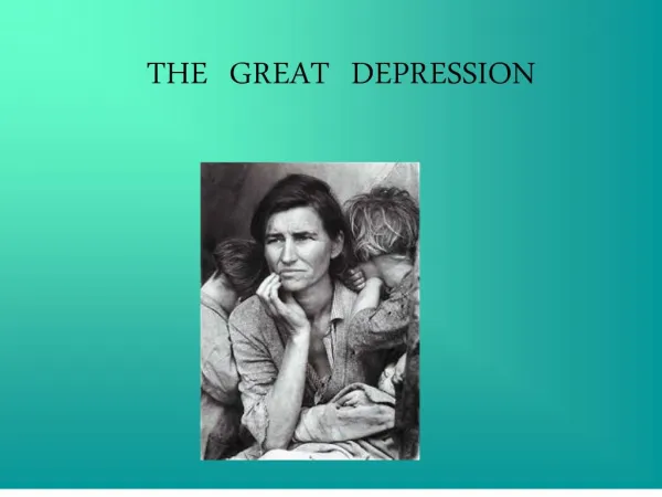
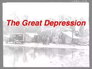
The Great Depression. Topic 12 Economics 2333 Robert A. Margo Spring 2013. Agenda. Background material Finegan and Margo Fishback , Horace, and Kantor Richardson and Troost. The Great Depression. Great Depression: Key macroeconomic e vent of the 20 th Century

palani
Download Presentation

The Great Depression

An Image/Link below is provided (as is) to download presentation Download Policy: Content on the Website is provided to you AS IS for your information and personal use and may not be sold / licensed / shared on other websites without getting consent from its author. Content is provided to you AS IS for your information and personal use only. Download presentation by click this link. While downloading, if for some reason you are not able to download a presentation, the publisher may have deleted the file from their server. During download, if you can't get a presentation, the file might be deleted by the publisher.

E N D

Presentation Transcript


  1. The Great Depression

    Topic 12 Economics 2333 Robert A. Margo Spring 2013
  2. Agenda Background material Finegan and Margo Fishback, Horace, and Kantor Richardson and Troost
  3. The Great Depression Great Depression: Key macroeconomic event of the 20th Century Impact of GD on economy + government policy was enormous, both short run and long run Also profound effect on economic theory: rise of Keynesian economics Vast macro research on explaining why the GD happened, depth, and recovery. Much focuses on US but some (very influential) is cross country (Eichengreen; Bernanke). Most influential recent work is Richardson and Troost. Ca. 1990 economic historians began to shift attention to microeconomic aspects of the GD. Most influential recent work is by Fishback and co-authors. Focuses on disaggregate effects of the New Deal, several papers.
  4. The Macroeconomy in the Long Run Steady upward trend with relatively brief short run instability (“business cycle) + GD GNP growth rate: average annual from 1870-present, about 3.2% per year with no acceleration Per capita income growth accelerated after WW2 Important business cycles before the GD: antebellum “panics” (1837-1843, 1857), late 1870s, mid-1880s, 1894 (the GD before the GD), 1908, post WWI (1921) Has the business cycle been tamed? Usual view is “yes” but this has been seriously challenged by Christina Romer in an important series of papers Romer argues that historical time series are “excessively” volatile due to data problems. Eg. historical unemployment. If we accept Romer’s criticisms (NOTE: not everyone does) the GD looms very large
  5. Basic Statistics Very sharp decline in nominal GNP Fall in price level but < nominal GNP so real GNP also falls NOT confined to US, (more or less) global event Stock market “crash” in 1929 Timing of changes well described by IP index Sharp rise in unemployment BUT real wages rise Dispute about evolution of unemployment after 1933: role of “work relief”
  6. Were We Prepared? Not really No unemployment insurance prior to 1930 “Welfare” had long existed, but was under the control of state and local governments Supplemented by private “relief” (eg. churches) Prior to GD, “unemployment” was largely seen as the individual’s fault Strong negative correlation between generosity of relief and % on relief prior to GD
  7. Key Questions Conventional debate: What Caused the GD? Monetarists vs. Keynes. NOTE: “freshwater” macro literature, too novel (IMHO) to judge. Why was it so prolonged? Role of the labor market vs. government policy What got the US out of the GD? New Deal or something else.
  8. What Caused the Great Depression? “Keynesian” view: stock market crash → exogenous drop in consumption (particularly durables) because uncertainty over future course of economy increases substantially Monetarist: minor business cycle turns into a major disaster because of inadequate response by Federal Reserve to drop in money supply Wave of bank failures, Fed response is too little, too late. Large negative external effects, see Bernanke. How to distinguish? Look at interest rates Temin (1976): If interest rate ↑, monetarist story has credibility but if interest rate ↓ then Keynesian story has credibility Nominal interest rates fall BUT we need to look at real rate of interest “Realized” real interest rates decline, also (Romer) expected real rate Key problem: there was deflation but was it anticipated? If expected change in price level is zero, then nominal rate = real rate If deflation was anticipated, real rate might have increased: debate is not settled
  9. Why was GD So Prolonged? Wage Rigidity: peculiar behavior of real wages and unemployment Some evidence of wage rigidity before GD BUT how much during 1930s is difficult to say because of compositional effects on unemployment. Least skilled/educated more likely to lose their jobs. Also (Ben Bernanke): role of work-sharing Possible disincentive effects of PEW work Policy errors. Recovery from 1933 is fairly robust, Fed pulls the plug too soon. Result is 1938 recession.
  10. Why Did it End? Fiscal Stimulus: Unlikely at macro level: Fed government was in full employment surplus in most years, state + local governments often raised taxes Micro level: some evidence that New Deal spending stimulated local retail sales – Fishback, et. al. External Demand is Key: rise of fascism in Europe (especially Germany) Capital inflows into US escaping Europe + war-related demand (prior to 1941)
  11. Long-Term Effects Substantial impact on government policy Shift of government spending from state/local to federal Expansion of federal spending: welfare, social security, unemployment insurance, “regulation”
  12. Finegan and Margo Famous debate in labor economics between W.S. Woytinsky (the originator of “human capital” theory) and Clarence Long. Context is late 1930s when the US is emerging from the GD. What will happen to the unemployment rate? Woytinsky believed there were many “added workers” who would exit so that unemployment would come down quickly. Long believed there were many “discouraged workers” who would enter the labor force but be unemployed for a while, causing the unemployment rate to remain high. Long was sure he was right. He cited a table from the 1940 census that showed the LFP of married women conditional on the employment status of their husbands. LFP was lower if husband was unemployed. Opposite of what Woytinsky predicted.
  13. Problems with Long’s argument In 1940 census persons on PEW (public emergency work) were technically deemed “unemployed”, as previously noted. HOWEVER in the table from the published 1940 census that Long cited, they were not separately distinguished from those who were truly unemployed, that is, without work of any kind. To get a PEW job, individuals had to be unemployed and their family income had to meet a “means” test. If family income was too high, they were unlikely to get a PEW job. PEW jobs were low wage but given prevailing social norms and gender gaps in pay, this might be better than looking for non-emergency work while wife continues to be in the LF. Strong incentive to working wives to drop out.
  14. Empirical Analysis How to test: (1) cross-section version of Long’s table BUT distinguish married men on PEW (2) use limited information in the 1940 census to infer something about transitions. Transitions in 1940 IPUMS. Individuals who worked in 1939 BUT who are not working during the 1940 census week. Or vice versa. Obviously imperfect but best that can be done with available data. Peculiarity of 1940 census. Individuals can be unemployed for 65 weeks as of late March 1940 BUT work 52 weeks in 1939. Income in 1939 includes income from work relief jobs.
  15. Tables 1-3 Table 1: IPUMS version of Long’s table. Note that wives of men on PEW were MUCH LESS likely to be in LF than either employed men or unemployed men. In March 1940, close to half of men who were “unemployed” according to the census definition were actually on work relief. If two LFPRs are averaged, the result is less than LFPR of married women whose husbands were employed. This is what Long saw in the published census table. Table 2: wives of husbands who were on PEW in March of 1940 were more likely to have worked in 1939 BUT were very likely to have exited during the first quarter of 1940. Table 3: multivariate versions of Table 1 and Table 2. Results are robust. Moral: even during the GD, labor market incentives matter.
  16. Fishback, Horace, and Kantor New Deal injected large amounts of money into local economies. Many different programs. What were the effects on recovery? FHK: report (in National Archives) documenting cumulative New Deal expenditures by county, 1933-1939, by program. Several papers. Best known is JEH 2005 on retail sales. Retail sales was used by the federal government to judge health of local economies in the 1930s. Data collected at periodic intervals. Basic finding: public works and relief spending clearly helped. Every dollar of same injected into local economies stimulated retail sales by about 44 cents. Suggests near 1-1 bounce in terms of per capita income. AAA spending, by contrast, seems to had either no effect, or possibly a negative effect.
  17. Richardson and Troost Bank failures were a big part of the GD. Differing views on the role of the Fed. One view is that the Fed failed to act quickly enough; a more activist monetary policy would have stemmed bank failures. Alternative view is that bank failures were “caused” by asset price declines and that the Fed at the time had limited ability to affect these. Previous work is either aggregate macro or else econometric with not much attention to identification. At the time the regional Feds had very different philosophies of helping out during bank crises. Fed district borders, however, were not the same as state borders. RT: examine Mississippi. One part of the state fell under the jurisdiction of the Atlanta Fed, the other under the jurisdiction of the St. Louis Fed. Atlanta Fed was interventionist, the St. Louis Fed was not. Look at what happens to banks in Mississippi on or near the Atlanta/St Louis border. Regression discontinuity design is common in labor and public economics but novel in macro.
  18. Data Panel data set of banks in Mississippi spanning the period. Information on bank characteristics and also whether they are in operation or go under. Linked to archival information on regional fed policies from minutes of meetings. Timeline of banking crisis can be documented from newspapers. Archival information on pre-GD banking crises reveals that Atlanta Fed was interventionist, while St. Louis Fed was not.
  19. Disaster Strikes November 7, 1930: Caldwell and Company collapses in Nashville. Caldwell was a large financial conglomerate with close ties to the Bank of Tennessee, which had many “correspondent” banks throughout the South. Correspondent banks fail BUT there were none in Mississippi. Instead, in Mississippi, the local business press reports news of financial distress. This appears to lead to bank runs. In the Atlanta district, the Fed intervenes, making funds available, but not in the St. Louis district. Leads to a simple prediction – less bank failure in the Atlanta district. Results consistent with this. Further, more bank failures → deeper downturn in local economy.
More Related