Download
1 / 19
190 likes | 333 Views
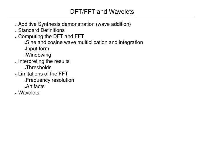
DFT/FFT and Wavelets. Additive Synthesis demonstration (wave addition) Standard Definitions Computing the DFT and FFT Sine and cosine wave multiplication and integration Input form Windowing Interpreting the results Thresholds Limitations of the FFT Frequency resolution Artifacts

E N D
DFT/FFT and Wavelets • Additive Synthesis demonstration (wave addition) • Standard Definitions • Computing the DFT and FFT • Sine and cosine wave multiplication and integration • Input form • Windowing • Interpreting the results • Thresholds • Limitations of the FFT • Frequency resolution • Artifacts • Wavelets
Summary of Demonstration • Complex waveforms are a summation of simple waves at differing frequencies • Each simple wave has two coefficients • Amplitude • Phase • Examining the time-domain waveform does not provide any real information about the coefficients: • Small changes in amplitude and phase can produce very different results in the time domain waveform • The DFT/FFT is a method that is designed to recover the simple waveform coefficients from a complex wave • The DFT/FFT makes a lot of assumptions
Definition • DFT: Discrete fourier transform • FFT: Optimized DFT. • Time-Domain waveform: A simple or complex waveform which is plotted wrt to time (x-axis) • Frequency domain: The data which represents the amplitude and phase of the series of simple waves which, when summed, produce a given complex waveform. Also called the “Spectrum”. • Amplitude: The peak value of a wave (either positive or negative) • Phase: The relation of a periodic waveform to its initial value expressed in factorial parts of the complete cycle. Usuall expressed as an angular measurement (0-360 degrees or 0-2*pi) • Stationary signals: Signals which maintain the same parameters over time. The FFT does not work well on non-stationary signals.
Computing the DFT • Given a sine wave: • Integrate the sine wave over 1 cycle • Result will be zero due to the symmetric nature of sine. • Take the same sine wave and multiple by itself. (ie. Squared) • The resulting waveform is no longer symmetric wrt the baseline • Integration will now yield a non-zero result • One can isolate a frequency component from any complex waveform by multipling the complex waveform by a simple waveform and then integrating. • If the integration yields a small result, we say that the frequency of the simple waveform is not a major component of the complex waveform • If the integration yields a large result, we say that the frequency of the simple waveform is a major component of the complex waveform
The FFT • The DFT involves many calculations involving complex numbers • N2 algorithm • Where N is the number of samples in the waveform • The FFT uses the “divide and conquer” approach • Involves breaking the N samples down into two N/2 sequences • Smaller sequences involve less computation and the recombination adds less overhead • Note: The FFT assumes that samples are equally spaced in time. • Because of the divide and conquer approach, N must be a power of 2. If your waveform does not have 2a samples, the waveform can be “padded” with zeros to fill up to 2a samples.
Sampling the waveform • Sine is a continuous function. The DFT/FFT works on discrete data • If you wish to perform an FFT on a continuous function, it is often most optimal to represent the continuous function in a discrete manner. • This process is called Sampling • As the function progresses in time, we can measure the distance between the function and some arbitrary baseline. (example on board) • This process yields a series of numbers which approximate the waveform. • Sampling can introduce artifacts/errors (example on board) • Sampling rate too small (Nyquist limit) • Not enough discrete levels
Real and Complex numbers • The definition of the DFT involves multiplying a complex signal by a sine wave. • If a major component of the complex waveform is equivalent the multiplied sine, the result is sin(x)2 • We need to take the square root of the integration, but the integration might yield a negative value • The result is that we need to use complex numbers to perform the computation. • Both the input and the output of the FFT include real an imaginary components.
Input to the FFT • Input to the FFT is an array of complex numbers which represents the input waveform • The complex portion is set to zero because the waveform exists in “real” space 0 1 2 3 ... Real Imaginary Real Imaginary ... Sample 1 Sample 2 ... Sample N 2N
Output from the FFT • The output of the FFT is an array of complex numbers which represents the spectrum • From each complex number we can compute: • Amplitude information • Phase information 0 1 2 3 ... Real Imaginary Real Imaginary ... 1st Harmonic (Positive Frequencies) 2nd Harmonic ... N/2 Harmonic (postive) N/2 Harmonic (negative) ... 2nd Harmonic 1st Harmonic (Negative Frequencies) 2N
Computing Amplitude and Phase • Plot the real and imaginary components on a plane (where one axis is the real component and the other is the imaginary component). • From the right angle triangle: Imaginary Axis • The amplitude is the hypotenuse • The phase is the angle (a) Real Imaginary Amplitude a Real Axis
Time localization • The FFT assumes that the signals are stationary. • The frequency components are present throughout the entire wave (from negative to positive infinity) • The phase components are present throughout the entire wave (from negative to positive infinity) • However, what happens when the wave is NOT stationary? • The FFT can tell you that the frequency is present, but it cannot tell you where the frequency exists in time within the wave (website pic) • Very few waveforms that exist within the real world are stationary. • If you do not care where in time the frequency exists, no problem. • If you do care where in time the frequency exists, you have to adjust how you use the FFT.
Windowing • Rather than analyse the whole waveform at once, we break the waveform down into discrete pieces. • This is called “Windowing” • Define a window which can hold N samples where N is a power of 2 • Copy the samples from time T within the original waveform into the window • Perform the FFT on the window • Slide the window over D samples and repeat the process (window slide) • The FFT will show which frequencies are present within the waveform from time T to (T+N samples) • We cannot localize within the window, but we can localize the window within the original waveform. • Unfortunately, windowing introduces artifacts • Solution: Use a windowing function: Hamming, Hanning, Kaiser-Bessel, Blackman, etc.
Windowing • When we apply a windowing function, we are (generally) trying to reduce high frequency artifacts which are introduced because of windowing. • In doing so, we are de-emphasizing the beginning and the end of the window. • When we slide the window, if we make the slide too large, we will lose information about the waveform. • The value for window slide is a power of 2 that is smaller than the window size. • ie. if we had a window size of 256 samples we would choose a slide value which is less than 128 samples • 64, 32, or 16 (typically)
Interpreting the results of the FFT • If we have a single window, we can simply plot the spectrum on a graph • The X axis is frequency • The Y axis is amplitude 50 40 Amplitude 30 20 10 100 200 300 Frequency
Interpreting the results of the FFT • If multiple FFTs have been performed, then the result is a 3 dimensional graph. • This graph is usually projected to 2 dimensional space where • The X axis is time • The Y axis is frequency • The intensity of the point is the amplitude • Some examples exist on the following site: http://pages.cpsc.ucalgary.ca/~hill/papers/synthesizer/index.html
Limitations of the FFT • The FFT produces approximate results. There are always artifacts introduced throughout the process • These artifacts manifest as noise within the spectrum • Filter out the noise using thresholds • The FFT does not deal well with discontinuities • Discontinuities manifest (typically) as high frequency noise in the spectrum • Because the FFT uses a single window size, the resolution is different for different frequencies. • You need a short window to capture high frequency components • You need a longer window to capture low frequency components
Wavelets • There are many similarities between wavelets and the FFT • They both attempt to factor a time-domain function into its spectrum • They both use translation functions to perform the factoring • Where wavelets differ from the FFT is precisely where the FFT has it's limitations • Wavelets are localized in space (ie. The wavelet translation function is localized) and thus work better with non-stationary signals • Wavelets have a scaling factor which provides better resolutions for differing frequencies
The Continuous Wavelet Transform • (Web Page) Formula • From the formula, we can see that there is a translation function (tao) and a scaling factor (s) • Tau defines the “mother wavelet”. • It is a local function • There are many different “mothers” to choose from. • Each mother tends to emphasize particular parts of the spectrum and de-emphasize other parts of the spectrum • The user needs to research which mother function is suitable to his/her application
The Scaling Factor • (Web Page) Diagram • When an FFT is performed, the window size remains constant. • This is why the FFT has different resolutions for different frequencies • Wavelets are applied with a changing window size. • The size of the window is called the “scale” • The variable “s” in the CWT definition causes the transform function to be “scaled” to differing sizes. • To obtain a clear definition of low frequency components, a large window is required • To obtain a clear definition of high frequency components, a small window is required • (web page diagram)