Download
1 / 41
420 likes | 697 Views
Grid design/boundary conditions and parameter selection. USGS publication (on course website): Guidelines for Evaluating Ground-Water Flow Models Scientific Investigations Report 2004-5038 http://www.usgs.gov/. NOTE:

E N D
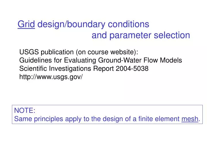
Grid design/boundary conditions and parameter selection USGS publication (on course website): Guidelines for Evaluating Ground-Water Flow Models Scientific Investigations Report 2004-5038 http://www.usgs.gov/ NOTE: Same principles apply to the design of a finite element mesh.
Finite Elements: basis functions, variational principle, Galerkin’s method, weighted residuals • Nodes plus elements; elements defined by nodes • Properties (K,S) assigned to elements • Nodes located on flux boundaries • Able to simulate point sources/sinks at nodes • Flexibility in grid design: • elements shaped to boundaries • elements fitted to capture detail • Easier to accommodate anisotropy that occurs at an • angle to the coordinate axis
Considerations in selecting the size of the nodal spacing in grid or mesh design Variability of aquifer characteristics (K,T,S) Variability of hydraulic parameters (R, Q) Kriging vs. zonation
Zonation Kriging
Considerations in selecting the size of the nodal spacing Variability of aquifer characteristics (K,T,S) Variability of hydraulic parameters (R, Q) Curvature of the water table Desired detail around sources and sinks (e.g., rivers)
Simulation of a pumping well Coarse Grid Fine Grid
Shoreline features including streams
Considerations in selecting the size of the grid spacing Variability of aquifer characteristics (K,T,S) (Kriging vs. zonation) Variability of hydraulic parameters (R, Q) Curvature of the water table Desired detail around sources and sinks (e.g., rivers) Vertical change in head (vertical grid resolution/layers)
Hydrogeologic Cross Section Need an average Kx,Kz for the cell
K1 K2 K3 Model cell is homogeneous and anisotropic Field system has isotropic layers Kx, Kz See eqns. 3.4a, 3.4b in A&W, p. 69, to compute equivalent Kx, Kz from K1, K2, K3.
anisotropy ratio K2 K1 4 m K2 K1
See Anderson et al. 2002, Ground Water 40(2) For discussion of high K nodes to simulate lakes
Capture zones 3D – 8 layer model 2D model
Orientation of the Grid • Co-linear with principal directions of K Finite difference grids are rectangular, which may result in inactive nodes outside the model boundaries. Finite element meshes can be fit to the boundaries.
Boundary Conditions Best to use physical boundaries when possible (e.g., impermeable boundaries, lakes, rivers) Groundwater divides are hydraulic boundaries and can shift position as conditions change in the field. If water table contours are used to set boundary conditions in a transient model, in general it is better to specify flux rather than head. > if transient effects (e.g., pumping) extend to the boundaries, a specified head acts as an infinite source of water while a specified flux limits the amount of water available. > You can switch from specified head to specified flux conditions as in Problem Set 6.
Treating Distant Boundaries 4 approaches General Head Boundary Condition Irregular grid spacing out to distant boundaries Telescopic Mesh Refinement Analytic Element Regional Screening Model
General Head Boundary (GHB) L Lake Model hB Q = C (hB - h) C = Conductance = K A/L K is the hydraulic conductivity of the aquifer between the model and the lake; A is the area of the boundary cell, perpendicular to flow.
Regular vs irregular grid spacing Irregular spacing may be used to obtain detailed head distributions in selected areas of the grid. Finite difference equations that use irregular grid spacing have a higher associated error than FD equations that use regular grid spacing. Same is true for finite element meshes.
Rule of thumb for expanding a finite difference grid: Maximum multiplication factor = 1.5 e.g., 1 m, 1.5 m, 2.25 m, 3.375 m, etc. In a finite element mesh, the aspect ratio of elements ideally is close to one and definitely less than five. The aspect ratio is the ratio of maximum to minimum element dimensions.
Treating Distant Boundaries General Head Boundary Condition Irregular grid spacing out to distant boundaries Telescopic Mesh Refinement Analytic Element Regional Screening Model
Using a regional model to set boundary conditions for a site model • Telescopic Mesh Refinement (TMR) • (USGS Open-File Report 99-238); • a TMR option is available in GW Vistas. • Analytic Element Screening Model
Using a regional model to set boundary conditions for a site model • Telescopic Mesh Refinement (TMR) • (USGS Open-File Report 99-238); • a TMR option is available in GW Vistas. • Analytic Element Screening Model
Review Types of Models • AnalyticalSolutions • Numerical Solutions • Hybrid (Analytic Element Method) • (numerical superposition of analytic solutions)
Review Types of Models • AnalyticalSolutions • Toth solution • Theis equation • etc… • Continuous solution defined by h = f(x,y,z,t)
Review Types of Models • Numerical Solutions • Discrete solution of head at selected nodal points. • Involves numerical solution of a set of algebraic • equations. Finite difference models (e.g., MODFLOW) Finite element models (e.g., MODFE: USGS TWRI Book 6 Ch. A3) See W&A, Ch. 6&7 for details of the FE method.
Finite Elements: basis functions, variational principle, Galerkin’s method, weighted residuals • Nodes plus elements; elements defined by nodes • Properties (K,S) assigned to elements • Nodes located on flux boundaries • Able to simulate point sources/sinks at nodes • Flexibility in grid design: • elements shaped to boundaries • elements fitted to capture detail • Easier to accommodate anisotropy that occurs at an • angle to the coordinate axis
Hybrid Analytic Element Method (AEM) Involves superposition of analytic solutions. Heads are calculated in continuous space using a computer to do the mathematics involved in superposition. The AE Method was introduced by Otto Strack. A general purpose code, GFLOW, was developed by Strack’s student Henk Haitjema, who also wrote a textbook on the AE Method: Analytic Element Modeling of Groundwater Flow, Academic Press, 1995. Currently the method is limited to steady-state, two-dimensional, horizontal flow
Theis solution assumes no regional flow. (from Hornberger et al. 1998) How does superposition work? Example: The Theis solution may be added to an analytical solution for regional flow without pumping to obtain heads under pumping conditions in a regional flow field.
Solution for regional flow. (from Hornberger et al. 1998) Apply principle of superposition by subtracting the drawdown calculated with the Theis solution from the head computed using an analytical solution for regional flow without pumping.
Using a regional model to set boundary conditions for a site model • Telescopic Mesh Refinement (TMR) • (USGS Open-File Report 99-238); • a TMR option is available in GW Vistas. • Analytic Element Screening Model
0 2 4 6 km Example: An AEM screening model to set BCs for a site model of the Trout Lake Basin Trout Lake Outline of the site we want to model N
Analytical element model of the regional area surrounding the Trout Lake site Outline of the Trout Lake MODFLOW site model Analytic elements outlined in blue & pink represent lakes and streams.
Flux boundary for the site model Results of the Analytic Element model using GFLOW
Water table contours from MODFLOW site model using flux boundary conditions extracted from analytic element (AE) model Flux boundaries Trout Lake
Particle Tracking east of Trout Lake Allequash Lake Big Muskellunge Lake Lakederived Terrestrial Simulated flow paths (Pint et. al, 2002)
Things to keep in mind when using TMR or an AEM screening models to set boundary conditions for site models • If you simulate a change in the site model that reflects • changed conditions in the regional model, you should • re-run the regional model and extract new boundary • conditions for the site model.
Example: Simulating the effects of changes in recharge rate owing to changes in climate Flux boundary for the site model might need to be updated to reflect changed recharge rates.
Things to keep in mind when using TMR or an AEM screening models to set boundary conditions for site models • If transient effects simulated in the site model extend • to the boundaries of the site model, you should re-run • the regional model under those same transient effects • and extract new boundary conditions for the site model for • each time step. Example: Pumping in a site model such that drawdown extends to the boundary of the site model.
TMR is increasingly being used to extract site models from regional scale MODFLOW models. • For example: • Dane County Model • Model of Southeastern Wisconsin • RASA models Also there is an AEM model of The Netherlands that is used for regional management problems. [deLange (2006), Ground Water 44(1), p. 111-115]