Download

1 / 39
390 likes | 494 Views
Business Cycles. What ar e we modelling ?. Focus on explaining fluctuations in real GDP, Y , and the GDP Deflator, P . Framework reminiscent of the supply and demand model. . SUPPLY. Two Aspects of Potential Output.

E N D
What are we modelling? • Focus on explaining fluctuations in real GDP, Y, and the GDP Deflator, P. • Framework reminiscent of the supply and demand model.
Two Aspects of Potential Output • Potential Output is unrelated to the price level but is determined by capital infrastructure, efficiency of labor markets, population, technological know-how. • Output increases above potential only if unemployment falls below natural level; • if unemployment rises above natural level, output will be below potential.
Potential output and labor market. • Potential output can be viewed as a level consistent with equilibrium in labor market. • When output is above potential output, low unemployment and the search for workers will push up wages. • When output is below potential, high unemployment and the surplus of workers will push down wages.
Potential Output YP P Unemployment above natural rate Unemployment below natural rate Upward Pressure on Wages Downward Pressure on Wages Y
Sticky Wages & SRAS • Money wages paid to workers adjust dynamically over time through negotiation. • At a given wage, a rise in the price level reduces the cost of labor relative to value of goods produced making hiring labor to produce goods more attractive. • At a given wage rate, higher prices induce higher production → in the short run, supply is positively associated with output.
Aggregate Supply Curve YP SRAS P Y
1. Shift in Potential Output • Advance in Technology Frontier, PP& E, or expansion in potential labor force (population, demographics). • Shifts SRAS w/ potential output. 2. Shifts in SRAS • When dollar cost of labor (or prices of energy) shift, changes in costs are passed on into prices. • Wages and other cost shifters shift SRAS at a given level potential output.
1. Expansion in Output Potential YP SRAS SRAS' YP ' P Y
2. Increase in Wages SRAS' YP P SRAS Y
Expenditure: C + I + G + NX • Wealth Effect – Real value of monetary assets rises as prices fall. This adds to wealth of households stimulating consumption. • Competitiveness Effect – Holding exchange rate constant, a lower price level makes domestic exports more attractive and foreign imports less stimulating net exports. Prices and Spending
Prices and Liquidity • Depending on monetary policy, there may be a negative relationship between prices and the liquidity that central banks make available. • More on that later.
Aggregate Demand Curve P AD Y
Equilibrium • Equilibrium in the competitive market occurs when the price is set at a level (P*) such that the amount that consumers want to buy is equal to the amount that sellers want to sell (Y*). Excess SupplyIf P were above equilibrium, sellers would want to sell more goods than buyers would want to buy. Competition between sellers would force prices down. Excess DemandIf P were below equilibrium, customers would want to buy more goods than people would want to sell. Competition between buyers would force prices up.
Equilibrium GDP and Price Level P SRAS P* AD Y Y*
Output below potential: Recessionary Gap. P YP AS 1 P* AD GAP Y Y*
Output above potential: Inflationary Gap. YP P AS 2 P* AD GAP Y Y*
Self Correction Process • Business cycles have a natural end. The equilibrium output may be greater than or less than potential output, however, in that case surplus or shortage of workers in labor markets will be putting downward or upward pressure on wages. • Pressure on wage costs will shift the supply curve until equilibrium output is equal to potential output.
AS1 YP P AS AS2 1 W↓ P* W↑ 2 AD Y Movement to Long Term Equilibrium
Cyclical Fluctuations • Period-by-period, different important events will impact the economy. We will think of these events as primarily driving the demand side of the economy (shifting the AD curve) or primarily driving the supply side (shifting the supply side). • The strength of these will determine the correspondence between movements in output and inflation.
Demand side shocks cause output and prices to move together. P AS P* 1 P** 2 AD1 AD2 Y Y** Y*
Output below potential. Downward pressure on wages. Cost of production falls and AS shifts down P YP AS AS2 1 As costs fall, competitive prices fall, there is a movement along the AD curve. Wages fall 2 3 P*** AD1 AD2 Y Y**
Wages will keep falling until the surplus of labor is absorbed – when prices fall enough that demand reaches potential output P AS2 AS4 P** 3 Wages fall 4 AD1 AD2 Y Y** YP
Consumer Confidence and… http://hk.nielsen.com/news/20091103.shtml http://business.asiaone.com/Business/News/Story/A1Story20091229-188708.html
..and Business Confidence… BNP Parabis Research
..and changes in Asset Prices.. http://urbanpolicy.berkeley.edu/pdf/CQSAdvMacro2005Web.pdf
AS-AD and Expected inflation • Potential GDP generally increases at a consistent rate. • On average, aggregate quantity of liquid assets tends to increase faster than potential GDP. • Workers wages will tend to rise to match increases in the cost of living. • AD does not always rise evenly with GDP.
Dynamic AS-AD Model: Trend Path YtP YPt+1 ASt ASt+1 P Demand expansion matches supply expansion P*t+1 Average Inflation Pt* ADt+1 ADt Y Yt* Y*t+1
Dynamic AS-AD Model: Inflation Acceleration YtP YPt+1 ASt+1 ASt P Demand expands faster than expected P*t+1 Expected Inflation Pt* Inflation rises more than usual ADt+1 ADt Positive Output Gap Gap Y Yt* Y*t+1
Dynamic AS-AD Model: Recession, Inflation Deceleration ASt+1 YPt+1 YtP ASt P Demand expands slower than expected P*t+1 Expected Inflation Pt* Inflation rises less than usual ADt+1 ADt Negative Output Gap Gap Y Yt* Y*t+1
Supply side shocks cause output and prices to move in opposite directions: Stagflation AS2 P AS 2 P** P* 1 AD1 Y Y** Y*
Bank of England Report Commodity Prices increase.. • In 2007, rising commodity & energy prices lead to global inflation
Learning Outcomes Students should be able to • Explain how various events will shift the aggregate supply or demand curves. • Construct an aggregate supply and demand model of business cycles and use it to explain equilibrium outcomes. • Describe the short-term and long-term dynamics of business cycles.