Download
1 / 25
250 likes | 255 Views
This article discusses the concept and benefits of path analysis using observed variables in social science research. It compares path analysis with multiple regression and highlights the advantages of path analysis with LISREL. The article also emphasizes the assumptions and considerations in conducting path analysis. Additionally, it explores the possibilities of model modification and provides examples of path models. Finally, the article touches upon the importance of sample size and discusses the concepts of mediation and moderation in path analysis.

E N D
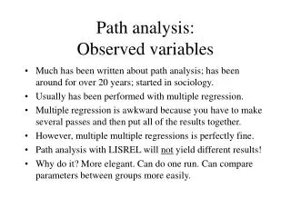
Path analysis:Observed variables • Much has been written about path analysis; has been around for over 20 years; started in sociology. • Usually has been performed with multiple regression. • Multiple regression is awkward because you have to make several passes and then put all of the results together. • However, multiple multiple regressions is perfectly fine. • Path analysis with LISREL will not yield different results! • Why do it? More elegant. Can do one run. Can compare parameters between groups more easily.
Assumptions • Multiple DVs: otherwise you’d just do a simple multiple regression • A single indicator for each measure (not latent). • Each variable is assumed to be perfectly reliable (no error). • Sufficient sample size: conservative estimate says at least 10 subjects per parameter; can sometimes get away with 5
Advantages • Forces you to explicitly state your model • Allows you to decompose your effects into direct and indirect effects • Can do model modification more easily: Remember, you must have a sufficiently large sample size to have exploratory and confirmatory samples
An example z1 X1 z3 Y1 b3,1 f1 g1,1 Y3 b2,1 b3,2 g2,1 Y2 z2
Details . . . • What is known and unknown? • Degrees of freedom = (N)(N+1)/2, or 10. • What is being estimated? One variance (phi for X1); 2 gammas; 3 betas; and 3 zetas = 9 unknowns. • Therefore, will run this path model with 1df.
. . . .details • Will focus on two chief matrices, first: Gamma: X1 Y1 free Y2 free Y3 0 (this is where we get 1df)
Beta matrix • Now the Beta matrix: Y1 Y2 Y3 Y1 --- --- --- Y2 free --- --- Y3 free free --- Note that the diagonal is non-meaningful; and that the top of the matrix is reserved for nonrecursive path models. In LISREL syntax, this matrix is called SD (or sub-diagonal).
Model fitting? • It is important to know that there will be no iterations. That means that there is no maximum likelihood generation of a latent variable (e.g., a ksi). • Still, the program does generate a host of fit indices to tell you whether your model fits the data well or not. Let’s look at this.
Path model of Mueller’s data z1 X1 g1,1 z3 Y1 b3,1 g1,2 f2,1 Y3 f3,1 b2,1 X2 g1,3 g2,1 g2,2 f3,2 g3,3 b3,2 X3 Y2 g2,3 z2
Now, with actual variables . . . z1 g1,1 z3 Mother Educ. Academic ability b3,1 g1,2 f2,1 Income 5 yrs. grad. f3,1 b2,1 Father Educ. g1,3 g2,1 g2,2 f3,2 g3,3 b3,2 Parent income Highest degree g2,3 z2
LISREL syntax: oh my, oh my Note: This is an observed path model on Mueller's data on college graduation DA NG=1 NI=15 NO=3094 MA=CM KM FI=a:\assign3\mueller.cor SD FI=a:\assign3\mueller.sds LA mothed fathed parincm hsrank desfin confin acaabil drvach selfcon degasp typecol colsel highdeg occpres incgrad se acaabil highdeg incgrad mothed fathed parincm/ MO NY=3 NX=3 PH=SY,FR PS=DI,FR GA=FU,FI BE=FU,FI FR GA(1,1) GA(1,2) GA(2,1) GA(2,2) GA(1,3) GA(2,3) GA(3,3)C BE(3,1) BE(3,2) BE(2,1) PD OU SC EF TV AD=50
the matrices . . . Gamma matrix: G X1X2 X3 Y1 free free free Y2 free free free Y3 0 0 free Beta matrix: B Y1Y2 Y3 Y1 ---- ---- ---- Y2 free ---- ---- Y3free free ----
How did the loadings turn out? .5* 2.6* .05* Mother Educ. Academic ability .07 .07* 1.1* Income 5 yrs. grad. .28* 1.5* Father Educ. .02 .01 .05* .01 2.1* .15* Parent income Highest degree .03* .86*
Measures of relative fit NFI = .99 RFI = .95 PNFI = .13 (not parsimonious) NNFI = .96 CFI = .99 Measures of absolute fit C2(2) = 19.98 GFI = 1.00 Critical N = 1426.88 RMSEA = .054 AGFI = .98 PGFI = .095 (i.e., not parsimonious) Model fit indices
Where do we go from here? • We obtained good model fit indices. . . alright, they’re damn good, except for parsimony. • Can we do better? Where can we trim the model? Delete the nonsignificant paths. This is model modification—do not attempt this without a confirmation sample, unless you want to claim that your model is merely exploratory.
New pruned model .5* 2.6* .06* Mother Educ. Academic ability .08* 1.1* Income 5 yrs. grad. .29* 1.4* Father Educ. .05* 2.1* .16* Parent income Highest degree .04* .86*
Measures of absolute fit C2(6) = 30.19 GFI = 1.00 Critical N = 1723.67 RMSEA = .036 (outstanding!) AGFI = .99 PGFI = .28 (better) Measures of relative fit NFI = .99 RFI = .98 PNFI = .40 (better) NNFI = .98 CFI = .99 Pruned model fit indices
How about a randomly generated model? .5* 2.6* .05* Income at grad. Mother Educ. .07 .07* 1.1* Academic ability .28* 1.5* Highest degree .02 .01 .05* .01 2.1* .15* Parent income Father Educ. .03* .86*
Measures of absolute fit C2(2) = 153.87 GFI = .98 Critical N = 186.16 RMSEA = .15 AGFI = .83 PGFI = .09 Measures of relative fit NFI = .95 RFI = .62 PNFI = .13 NNFI = .62 CFI = .95 Fit for randomly generated model
Moral of the story • Some indices are affected more than others • When you have a huge sample size, and a host of correlated measures, you’ll still end up with some acceptable fit indices. So beware! • With smaller sample sizes and stinky variables (low internal reliability), covariances will be smaller, and model fit will suffer accordingly. So, don’t get used to a sample size of 3,000.
Mediation or moderation? • All of the models proposed thus far have featured mediation: A => B => C. • As you probably know, I like moderation too. Much confusion over which to use. • Baron & Kenny’s rules: must have sig. covariation between all variables before attempting. Not always obtained. • So how would one do moderation?
Mediation and moderation Stress Coping Outcome Stress Outcome Coping
Statistically, how are they different or similar? • Both can be performed on either observed or latent (although a moderational path model has not been standardized yet). • We’ve seen the mediation model, let’s consider the moderation model. • The chief issue is that there is one Y variable (outcome), and all other variables are considered to be X variables.
The figure Stress Outcome Coping Stress X Coping
Syntax Note: This is an observed path model for the moderation of stress on outcome by coping DA NG=1 NI=4 NO=0 MA=CM KM FI=a:\stress.dat LA stress coping strxcop outcome se outcome stress coping strxcop/ MO NY=1 NX=3 PH=SY,FR PS=DI,FR GA=FU,FI FR GA(1,1) GA(2,1) GA(3,1) PD OU SC EF TV AD=50