Statistical Water Supply (SWS)

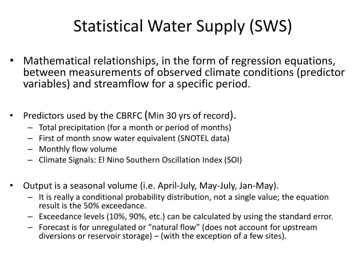
1. Statistical Water Supply (SWS) • Mathematical relationships, in the form of regression equations, between measurements of observed climate conditions (predictor variables) and streamflow for a specific period. • Predictors used by the CBRFC (Min 30 yrs of record). • Total precipitation (for a month or period of months) • First of month snow water equivalent (SNOTEL data) • Monthly flow volume • Climate Signals: El Nino Southern Oscillation Index (SOI) • Output is a seasonal volume (i.e. April-July, May-July, Jan-May). • It is really a conditional probability distribution, not a single value; the equation result is the 50% exceedance. • Exceedancelevels (10%, 90%, etc.) can be calculated by using the standard error. • Forecast is for unregulated or “natural flow” (does not account for upstream diversions or reservoir storage) – (with the exception of a few sites).

2. Calculation Example: Flow observed at stream gage is adjusted for upstream diversions and/or reservoir storage. This procedure is done for all historical data and used in equation development, and forecast verification. June 2010 calculation RRBPC2 QCMPAZZ 06-2010 OBS AVG %AVG RBPC2 QCMRZZZ + 1.66A 7.55 22% BDVC2 QCMRZZZ + 12.36A 12.00 103% -------------- 14.02A 18.35 76% NAVC2 QCMPAZZ 06-2010 OBS AVG %AVG NAVC2 QCMRZZZ + 4.64A 8.83 53% NOSC2 QCMRZZZ + 14.61A 15.32 95% -------------- 19.25A 24.74 78% FRMN5 QCMPAZZ 06-2010 OBS AVG %AVG FRMN5 QCMRZZZ + 117.89Z 289.82 41% NVRN5 LSMRZZZ + 38.37A 63.79 60% CHUN5 QCMRZZZ + 27.58A 30.05 92% VCRC2 LSMRZZZ + 3.13A 16.45 19% LEMC2 LSMRZZZ + -3.21A 4.45 -72% NIIN5 QCMRZZZ + 39.83A 26.75 149% DPPC2 QCMRZZZ + 15.36A 0.00 -999 -------------- 238.96A 426.85 56%

3. Source: NRCS Developing Equations: Predictor variables must make sense Challenge when few observation sites exist within river basin Challenge when measurement sites are relatively young Fall & Spring precipitation is frequently used (why?) Trial Lake SNOTEL • Sample Equation for April 1: April-July volume Weber @ Oakley = + 3.50 * Apr 1st Smith & Morehouse (SMMU1) Snow Water Equivalent + 1.66 * Apr 1st Trial Lake (TRLU1) Snow Water Equivalent + 2.40 * Apr 1st Chalk Creek #1 (CHCU1) Snow Water Equivalent - 28.27

4. Statistical Water Supply (SWS) • Two types of forecast equations: • Headwater Equations: Previous example using current climate measures for predictor variables (typically top of basin sites) • Routed Equations: For downstream points the regression equation‘routes’ the upstream volume forecast. A relationship is built between historical observed runoff between upstream and downstream sites. The upstream forecast volume is then plugged into this relationship resulting in a forecast for the downstream site. • Routed Forecast Equation Example: Lake Powell • Good correlation with historical upstream observed flows: • Green at Green River + Colorado nr Cisco + San Juan nr Bluff • r2 = .994 for historical observed data between Powell and these sites • Forecast at these upstream sites are plugged into this relationship

5. SWS Software Demonstration: PSPC2: San Juan @ Pagosa Springs – Headwater Equation NVRN5: San Juan, Navajo Reservoir Inflow – Routed Equation

12. Easy to calibrate, maintain and run, but requires sufficient historical record. Does not represent physical processes associated with snow melt, runoff, etc. Developed only for seasonal volumes (pre-defined periods in equations). Equations can only be run at specific times (i.e. first of month) for a specific forecast period. Lacks representation of soil moisture Requires extensive calibration, maintenance, & infrastructure. Stringent data requirements. Physical processes represented mathematically. Can compute many hydrologic variables over any period. Can be run at any time for any period. Keeps track of soil moisture. SWS vs. ESP