Download
1 / 48
480 likes | 607 Views
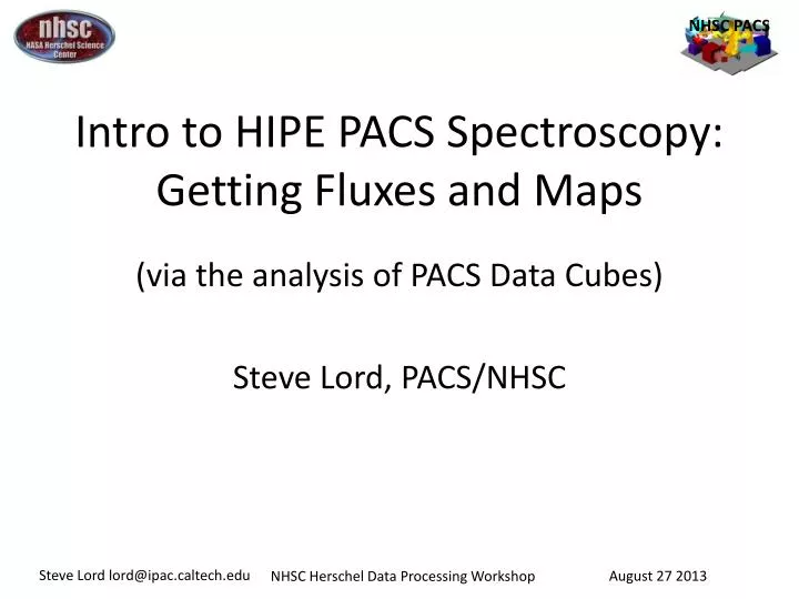
Intro to HIPE PACS Spectroscopy: Getting Fluxes and Maps. (via the analysis of PACS Data Cubes) Steve Lord, PACS/NHSC. We will stay in the safety of Level 2, out of the deep water. Level 2.5 Level 2 Level 1 Level 0. We will assume the automatic processing worked well….

E N D
Intro to HIPE PACS Spectroscopy: Getting Fluxes and Maps (via the analysis of PACS Data Cubes) Steve Lord, PACS/NHSC
We will stay in the safety of Level 2, out of the deep water Level 2.5 Level 2 Level 1 Level 0
We will assume the automatic processing worked well…. But the subsequent talks will go deeper…..
PACS Fundamentals • The PACS spectrograph is an IFU with a field of view of approximately 47”x47” covered with an 5 x 5 array. The pixels are fixed at 9.4” sampling. • The spectrograph covers wavelengths from 55 to 210μm • The spatial image is sliced in 5 rows and each is dispersed along an array of 16 spectral pixels. • Observations are executed by moving the grating inoverlapping increments to scan the requested wavelength range, leading to a high degree of redundancy. • A region of sky may be covered in multiple footprints yielding a raster map. • Reduced data are arranged into cubes of two spatial dimensions and one wavelength dimension for visualization and analysis.
Spectral Resolution vs. Wavelength A Herschel resolution vs. wavelength comparison
Spectral Resolution vs. Lambda Herschel Spitzer
Spatial Resolution vs. LambdaWhen interpreting maps, consider: Source Size, Instrument Resolution, and Pixel Size PACS Spectrometer Beam Point Spread Function Pixel Size = 9.4" Adjacent Pixels fully sample images, and over-sample long wavelength images PACS Observer Manual Fig 4.2
PACS Spectroscopy Observing Modes Calibration: Chopped or Unchopped Mapping: Single Point, Dithered, or Rastered Bandwidth: Lines, Small Ranges, Large Ranges
Cube Types Reflect the Processing “Projected Cubes” “PACS Cubes” “Frame” Arrays “Rebinned Cubes” Frame Arrays: Data are observed as (25 x 16) frames resulting in (25 x 16 x Nframes ) arrays. PACS Cubes: The pipeline reorganizes data into a cube with two spatial and one λdimension. LEVEL 2: Rebinned Cubes: (5 x 5 x λ) cube is rebinned into a (5 x5 x Nλ) cube; one per pointing. Projected Cubes: (Nx x Ny x Nλ ) data are projected on a spatial Nx x Ny RA-Dec grid. Level 2…….
Important Initial Analysis Decision:Deciding whether to use*Rebinned Cubes*or *Projected Cubes*
Why does it matter? • You want to use the correct final product for your fluxes and spectra – depending on the observation, the correct final product is either a Rebinned Cube or a Projected Cube. • Both cube types are present in each data set. You must know how to decide which you need and where to find it. You want to spend your time working with the right cube to cull out specific measurements.
"When to Use Which Cube" GUIDE Projected Cube: One or more Rebinned Cubes that has been Projected (Mosaicked) together onto RA & Dec Coordinates. Rebinned Cubes: The PACS 5x5 Spatial Footprint x a Wavelength Axis. λ λ λ 3" pixels typically y Dec λ z RA 9.4" pixels Extended Sources Point Sources
For Sampling Quality – Consider Overlap Under Sampled Poorly Sampled > Nyquist Sampled
The Actual Footprint (the centers)This is the Rebined Cube-face on the sky Red and Blue Array Poglitch et al. 2010 A&A 518 L2 There is no excellent beauty that hath not some strangeness in the proportion.” – Francis Bacon
PACS Footprint Viewer Script(very simple – 4 lines) # Bring in an Image with a valid FITS WCS (RA Dec) M82_image = fitsReader(file = '/Users/lord/Desktop/NGC_3034-I-Ha-kab2003.fits') # Start up the application by loading the image in footprintApi = pacsSpectralFootprint(input=M82_image) # grab a rebinned cube of interest (can ve dragged from the level list to the variable list) pacsrebinnedcube = obs99.refs["level2"].product.refs["HPS3DRB"].product.refs[0].product # Overlay the outline of the footprint pixels footprintApi.addFootprint(pacsrebinnedcube) # rt. click to zoom
Where to Find Spectrum Explorer Documentation • PACS Data Reduction Guide: Spectroscopy Sect 8.5 (a meager amount of content) • Best: The Data Analysis Guide: • Chapter 6: The Spectrum Explorer • Chapter 7: Line Fitting • (It’s all there….)
Some Things that Spectrum Explorer Can Do • Make Continuum Maps • Make Moment Maps • (e.g., velocity) • View Residuals • Average Cube regions • Produce Basic Products • Unit Conversion (indirectly) • Visualize w/Three Panels: Select, Preview, and Display • Crop Spatially • Crop Spectrally • Fit Lines • Fit Multi-Gaussians • Fit the Entire Cube
Projected and Rebinned Cubes Herschel PACS Spec. 3 D Data Projected Red Herschel PACS Spec. 3 D Data RebinnedRed Click for Spectrum Explorer
Rebinned Cube Wavelength Slide Zoom Controls
Projected Cube Organization of the Spectrum Explorer Image Display Panel, Preview Panel, Spectral Display, additional tasks panel…….
Projected Cube Mosaic Spectra
Saving Integrated Intensity Maps - I First: Make Model Component Cubes with Multi-Fit option of Spectrum Fitted GUI Multi-fit makes model component cubes
Saving Integrated Intensity Maps - II Second Step: Integrate Model-Component Cube with Cube Spectral Analysis Task We have integrated a model component (the redshifted Gaussian) over a wavelength range to produce a 2-d integrated flux map shown. It may be saved to FITS.
Making a Velocity Map - 1 First of all, let display the cube with SE and click on a pixel
Select ranges Making a Velocity Map - 3 Click on the icon and, with click and drag, select two ranges ...
Making a Velocity Map - 4 Press “Accept” and two new cubes will appear (sub & base) ….
Making a Velocity Map - 5 We will go back to “Variables” to select the subCube ….
Making a Velocity Map - 6 Then, we will select the subCube by right-clicking on its name to open it with Spectrum Explorer.
Making a Velocity Map - 7 Open SE again and select “computeVelocityMap” ….
Making a Velocity Map - 8 Select MOMENTS, write the reference wavelength and Accept !
Making a Velocity Map - 9 A series of new cubes is created, including the velocity map ...
Making a Velocity Map - 10 Output the”SimpleImage “ Velocity Map to aFIX Export in Fits as SimpleImage -
Alternative Spatial Projections: “Drizzled Cubes” Drizzled cubes are not yet a standard archive product – but theylikely will become one in the future.
Why Drizzling? • The alternative, specProject allows the wavelength grid and outlier detection to occur before the projection task. It gives a quick and basically correct answer • Drizzle goes back to the pacsCubes before wavelength binning and thus captures the spectral information before binning • It also captures the spatial information present in each wavelength before rebinning • Likewise it handles the Two nod position’s spatial variations in its processing • Finally by “shrinking” the detector flux – the so called “droplets of the drizzle, it minimizes the effect of each spaxels footprint that typically underfills the beam point spread function
When Drizzle Helps.... • This spatial projection method (like specProject) combines the data from overlapping points of a raster map, placing emission onto a uniform spatial grid in a World Coordinates System. • The method is appropriate for spatially oversampled observations. (Consider the 9.4” “native” sampling and the resolution at the line wavelength for this determination). • The method always requires large memory and is computationally intensive. • It can be applies only over narrow wavelength ranges (line or small range spectroscopy modes) over a few microns or less. • Yet it is the preferred method projection method when all of the above requirements are met.
Droplets The flux is shrunk to the inner squares (“drops”) and then drizzled down in smaller quantities (“droplets”) to the output pixels below.
The pacsCubes are used for the drizzling. This bypasses the wavelength binning typically done to make rebinned cubes PACS PIPELINE CUBE BUILDING SINGS background RAW Level 0 To Level 0.5 Projected to 3” x 3” pixels To calibrated L1 FRAMES CALIBRATED PACSCUBE Level 1 data data
Setting the parameters • The 1st 4 parameters are integer. • oversampleWave – the wavelength binsize in units of the spectral resolution element. overSample=2 is Nyquist sampling. • upsampleWave – The number of bins per binsize. E. g., upsample=2 implies doubling the number of bins through overlapping them. (examples follow) • overSampleSpace – this is in units of the telescope resolution. overSampleSpace=2 is Nyquist Sampling • upSampleSpace – this is the 2d spatial analog of upSample wave • picFrac – this is the spatial “shrinking” factor of the flux on the originating pixel to spatially limit the flux origin to an area smaller than the pixel footprint
Example Code • # DRIZZLING • # Drizzling is new from hipe 10.0. It works from the not-rebinned PacsCubes • ### CREATE WAVELENGTH AND SPATIAL GRIDS • # For an explanation of the parameters of wavelengthGrid, spatialGrid and drizzle, • # see the PACS spectroscopy data reduction guide • # Recommended values for oversampleSpace and upsampleSpace are 3 and 2 respectively • # Recommended value for pixFrac is >= 0.3 for oversampled rasters, and >= 0.6 for Nyquist sampled rasters • # The raster step sizes can be found in meta data entries 'lineStep' and 'pointStep' • oversampleWave = 2 • upsampleWave = 3 • waveGrid = wavelengthGrid(slicedCubes, oversample=oversampleWave, upsample=upsampleWave, calTree = calTree) • oversampleSpace = 3 • upsampleSpace = 2 • pixFrac = 0.6 • spaceGrid = spatialGrid(slicedCubes, wavelengthGrid=waveGrid, oversample=oversampleSpace, upsample=upsampleSpace, pixfrac=pixFrac, calTree=calTree) • ### DRIZZLE • slicedDrizzledCubes = drizzle(slicedCubes, wavelengthGrid=waveGrid, spatialGrid=spaceGrid) • # Save drizzled cubes to pool • # name = "OBSID_"+str(obsid)+"_"+camera+"_slicedDrizzledCubes" • # saveSlicedCopy(slicedDrizzledCubes,name) • # if updateObservationContext: obs = updateObservation(obs, camera, "2", slicedRebinnedCubes=slicedFinalCubes, projectedCube=slicedDrizzledCubes) Method of saving Drizzle Products
Resources for PACS Spectral Analysis • Videos: • Webinars (recorded) • Manuals: PACS Spec, Data Reduction Guide Sect 6.4 • Also see – • the General Data Analysis Guide Chapters 6 and 7 • Tutorials: https://nhscsci.ipac.caltech.edu/sc/index.php/Pacs/DataProcessing https://nhscsci.ipac.caltech.edu/sc/index.php/Pacs/DataProcessing
Wavelength Offsets due to pointing Errors or Offsets(From the PACS Observers Manual, in partial answer to a User Question in the Webinar)
Extending a PACS SED through to SPIRE A resolution vs. wavelength guide At 200 um, PACS and SPIRE overlap a little, and also have similar spectral resolution. Further, 3x3 PACS Spaxels are about the size of one SPIRE Pixel. Stitching SEDs is however hampered by the PACS order leak at 190-220 um, making calibration difficult to Achieve.