Download
1 / 46
460 likes | 555 Views
Database Systems I SQL Queries. Introduction. We now introduce SQL, the standard query language for relational DBS. As RA, an SQL query takes one or two input tables and returns one output table. Any RA query can also be formulated in SQL, but in a more user-friendly manner.

E N D
Introduction • We now introduce SQL, the standard query language for relational DBS. • As RA, an SQL query takes one or two input tables and returns one output table. • Any RA query can also be formulated in SQL, but in a more user-friendly manner. • In addition, SQL contains certain features of great practical importance that go beyond the expressiveness of RA, e.g. sorting and aggregation functions.
Example Instances R1 S1 • We will use these instances of the Sailors and Reserves tables in our examples. S2
Basic SQL Query SELECT [DISTINCT] target-list FROMrelation-list WHERE qualification • relation-list: list of relation names (possibly with a tuple-variable after each name). • target-list: list of attributes of relations in relation-list • qualification : comparisons (“Attr op const” or “Attr1 op Attr2”, where op is one of ) combined using AND, OR and NOT. • DISTINCT is an optional keyword indicating that the answer should not contain duplicates. Default is that duplicates are not eliminated!
Conceptual Evaluation Strategy • Semantics of an SQL query defined in terms of the following conceptual evaluation strategy: • Compute the Cartesian product of relation-list. • Selection of the tuples satisfying qualifications. • Projection onto the attributes that are in target-list. • If DISTINCT is specified, eliminate duplicate rows. • This strategy is not an efficient way to process a query! An optimizer will find more efficient strategies to compute the same answers. • It is often helpful to write an SQL query in the same order (FROM, WHERE, SELECT).
Example Conceptual Evaluation SELECT S.sname FROM Sailors S, Reserves R WHERE S.sid=R.sid AND R.bid=103
Projection Expressed through the SELECT clause. Can specify any subset of the set of all attributes. SELECT sname, age FROM Sailors; “*” selects all attributes.SELECT * FROM Sailors; Can rename attributes.
Projection • For numeric attribute values, can also apply arithmetic operators +, * etc. • Can create derived attributes and name them, using AS or “=“: • SELECT age AS age0, age1=age-5, 2*S.age AS age2 • FROM Sailors;
Projection • The result of a projection can contain duplicates (why?). • To eliminate duplicates from the output, specify DISTINCT in the SELECT clause. SELECT DISTINCT age FROM Sailors;
Selection Expressed through the WHERE clause. Selection conditions can compare constants and attributes of relations mentioned in the FROM clause. Comparison operators: =, <>, <, >, <=, >= For numeric attribute values, can also apply arithmetic operators +, * etc. Simple conditions can be combined using the logical operators AND, OR and NOT. Default precedences: NOT, AND, OR. Use parentheses to change precedences.
Selection SELECT * FROM Sailors WHERE sname = ‘Watson’; SELECT * FROM Sailors WHERE rating >= age; SELECT * FROM Sailors WHERE (rating = 5 OR rating = 6) AND age <= 20;
String Comparisons • LIKE is used for approximate conditions (pattern matching) on string-valued attributes: string LIKE pattern • Satisfied if pattern contained in string attribute. • NOT LIKE satisfied if pattern not contained in string attribute. • ‘_’ in pattern stands for any one character and ‘%’ stands for 0 or more arbitrary characters. SELECT * FROM Sailors S WHERE S.sname LIKE ‘B_%B’;
Null Values • Special attribute value NULL can be interpreted as: • Value unknown (e.g., a rating has not yet been assigned), • Value inapplicable (e.g., no spouse’s name), • Value withheld (e.g., the phone number). • The presence of NULL complicates many issues: • Special operators needed to check if value is null. • Is rating>8 true or false when rating is equal to null? What about AND, OR and NOT connectives? • Meaning of constructs must be defined carefully. E.g., how to deal with tuples that evaluate neither to TRUE nor to FALSE in a selection?
Null Values • NULL is not a constant that can be explicitly used as an argument of some expression. • NULL values need to be taken into account when evaluating conditions in the WHERE clause. • Rules for NULL values: • An arithmetic operator with (at least) one NULL argument always returns NULL. • The comparison of a NULL value to any second value returns a result of UNKNOWN. • A selection returns only those tuples that make the condition in the WHERE clause TRUE, those with UNKNOWN or FALSE result do not qualify.
Truth Value Unknown Three-valued logic: TRUE, UNKNOWN, FALSE. Can think of TRUE = 1, UNKNOWN = ½, FALSE = 0. AND of two truth values: their minimum. OR of two truth values: their maximum. NOT of a truth value: 1 – the truth value. Examples: TRUE AND UNKNOWN = UNKNOWN FALSE AND UNKNOWN = FALSE FALSE OR UNKNOWN = UNKNOWN NOT UNKNOWN = UNKNOWN
Truth Value Unknown • SELECT * • FROM Sailors • WHERE rating < 5 OR rating >= 5; • Does not return all sailors, but only those with non-NULL rating.
Ordering the Output • Can order the output of a query with respect to any attribute or list of attributes. • Add ORDER BY clause to the query: SELECT * FROM Sailors S WHERE age < 20 ORDER BY rating; SELECT * FROM Sailors S WHERE age < 20 ORDER BY rating, age; • By default, ascending order. Use DESC to specify descending order.
Cartesian Product • Expressed in FROM clause. • Forms the Cartesian product of all relations listed in the FROM clause, in the given order. SELECT * FROM Sailors, Reserves; • So far, not very meaningful.
Join • Expressed in FROM clause and WHERE clause. • Forms the subset of the Cartesian product of all relations listed in the FROM clause that satisfies the WHERE condition: SELECT * FROM Sailors, Reserves WHERE Sailors.sid = Reserves.sid; • In case of ambiguity, prefix attribute names with relation name, using the dot-notation.
Join • Since joins are so common operations, SQL provides JOINas a shorthand. SELECT * FROM Sailors JOIN Reserves ON Sailors.sid = Reserves.sid; • NATURAL JOIN produces the natural join of the two input tables, i.e. an equi-join on all attributes common to the input tables. SELECT * FROM Sailors NATURAL JOIN Reserves;
Join • Typically, there are some dangling tuples in one of the input tables that have no matching tuple in the other table. Dangling tuples are not contained in the output. • Outer joins are join variants that do not loose any information from the input tables: • LEFT OUTER JOIN includes all dangling tuples from the left input table with NULL values filled in for all attributes of the right input table. • RIGHT OUTER JOIN includes all dangling tuples from the right input table with NULL values filled in for all attributes of the left input table. • FULL OUTER JOIN includes all dangling tuples from both input tables.
Tuple Variables • Tuple variable is an alias referencing a tuple from the relation over which it has been defined. • Again, use dot-notation. • Needed only if the same relation name appears twice in the query. SELECT S.sname FROM Sailors S, Reserves R1, Reserves R2 WHERE S.sid=R1.sid AND S.sid=R2.sid AND R1.bid <> R2.bid • It is good style, however, to use tuple variables always.
A Further Example • Find sailors who’ve reserved at least one boat: SELECT S.sid FROM Sailors S, Reserves R WHERE S.sid=R.sid • Would adding DISTINCT to this query make a difference? • What is the effect of replacing S.sid by S.sname in the SELECT clause? What about adding DISTINCT to this variant of the query?
Set Operations • SQL supports the three basic set operations. • UNION: union of two relations • INTERSECT: intersection of two relations • EXCEPT: set-difference of two relations • Two input relations must have same schemas. Can use AS to make input relations compatible.
Set Operations • Find sid’s of sailors who’ve reserved a red or a green boat. • If we replace OR by AND in the first version, what do we get? • What do we get if we replace UNION by EXCEPT? SELECT S.sid FROM Sailors S, Boats B, Reserves R WHERE S.sid=R.sid AND R.bid=B.bid AND (B.color=‘red’ OR B.color=‘green’); (SELECT S.sid FROM Sailors S, Boats B, Reserves R WHERE S.sid=R.sid AND R.bid=B.bid ANDB.color=‘red’) UNION (SELECT S.sid FROM Sailors S, Boats B, Reserves R WHERE S.sid=R.sid AND R.bid=B.bid ANDB.color=‘green’);
Set Operations SELECT S.sid FROM Sailors S, Boats B1, Reserves R1, Boats B2, Reserves R2 WHERE S.sid=R1.sid AND R1.bid=B1.bid AND S.sid=R2.sid AND R2.bid=B2.bid AND (B1.color=‘red’ AND B2.color=‘green’); • Find sid’s of sailors who’ve reserved a red and a green boat. • Contrast symmetry of the UNION and INTERSECT queries with how much the other versions differ. Key attribute! (SELECT S.sid FROM Sailors S, Boats B, Reserves R WHERE S.sid=R.sid AND R.bid=B.bid AND B.color=‘red’) INTERSECT (SELECT S.sid FROM Sailors S, Boats B, Reserves R WHERE S.sid=R.sid AND R.bid=B.bid AND B.color=‘green’);
Subqueries • A subquery is a query nested within another SQL query. • Subqueries can • return a a single constant that can be used in the WHERE clause, • return a relation that can be used in the WHERE clause, • appear in the FROM clause, followed by a tuple variable through which results can be referenced in the query. • Subqueries can contain further subqueries etc., i.e. there is no restriction on the level of nesting.
Subqueries • The output of a subquery returning a single constant can be compared using the normal operators =, <>, >, etc. SELECT S.age FROM Sailors S WHERE S.age > (SELECT S.age FROM Sailors S WHERE S.sid=22); • How can we be sure that the subquery returns only one constant? • To understand semantics of nested queries, think of a nested loops evaluation: For each Sailors tuple, check the qualification by computing the subquery.
Subqueries • The output of a subquery R returning an entire relation can be compared using the special operators • EXISTS Ris true if and only if R is non-empty. • s IN Ris true if and only if tuple (constant) s is contained in R. • s NOT IN Ris true if and only if tuple (constant) s is not contained in R. • s op ALL Ris true if and only if constant s fulfills op with respect to every value in (unary) R. • s op ANY Ris true if and only if constant s fulfills op with respect to at least one value in (unary) R. • Op can be one of
Subqueries • EXISTS, ALL and ANY can be negated by putting NOT in front of the entire expression. SELECT R.bid FROM Reserves R WHERE R.sid IN (SELECT S.sid FROM Sailors S WHERE S.name=‘rusty’); SELECT * FROM Sailors S1 WHERE S1.age > ALL (SELECT S2.age FROM Sailors S2 WHERE S2.name=‘rusty’);
Subqueries • In a FROM clause, we can use a parenthesized subquery instead of a table. • Need to define a corresponding tuple variable to reference tuples from the subquery output. SELECT * FROM Reserves R, (SELECT S.sid FROM Sailors S WHERE S.age>60) OldSailors WHERE R.sid = OldSailors.sid;
Correlated Subqueries SELECT B.bid FROM Boats B WHERE NOT EXISTS (SELECT * FROM Reserves R WHERE R.bid=B.bid); • The second subquery is correlated to the outer query, i.e. the execution of the subquery may return different results for every tuple of the outer query. • Illustrates why, in general, subquery must be re-computed for each tuple of the outer query / tuple.
A Further Example • Find sid’s of sailors who’ve reserved both a red and a green boat: SELECT S.sid FROM Sailors S, Boats B, Reserves R WHERE S.sid=R.sid AND R.bid=B.bid AND B.color=‘red’ AND S.sid IN (SELECT S2.sid FROM Sailors S2, Boats B2, Reserves R2 WHERE S2.sid=R2.sid AND R2.bid=B2.bid AND B2.color=‘green’); • Similarly, EXCEPT queries re-written using NOT IN. • To find names (not sid’s) of Sailors who’ve reserved both red and green boats, just replace S.sid by S.sname in SELECT clause. (What about INTERSECT query?)
Division in SQL • Find sailors who’ve reserved all boats. • With EXCEPT: SELECT S.sname FROM Sailors S WHERE NOT EXISTS ((SELECT B.bid FROM Boats B) EXCEPT (SELECT R.bid FROM Reserves R WHERE R.sid=S.sid));
Division in SQL • Find sailors who’ve reserved all boats. • Without EXCEPT: SELECT S.sname FROM Sailors S WHERE NOT EXISTS(SELECT B.bid FROM Boats B WHERE NOT EXISTS(SELECT R.bid FROM Reserves R WHERE R.bid=B.bid AND R.sid=S.sid)) Sailors S such that ... there is no boat B without ... a Reserves tuple showing S reserved B
Aggregation Operators • Operators on sets of tuples. • Significant extension of relational algebra. • COUNT (*): the number of tuples. • COUNT ( [DISTINCT] A): the number of (unique) values in attribute A. • SUM ( [DISTINCT] A): the sum of all (unique) values in attribute A. • AVG ( [DISTINCT] A): the average of all (unique) values in attribute A. • MAX (A): the maximum value in attribute A. • MIN (A): the minimum value in attribute A.
Aggregation Operators (4) SELECT S.sname FROM Sailors S WHERE S.rating= (SELECT MAX(S2.rating) FROM Sailors S2); (5) SELECT AVG ( DISTINCT S.age) FROM Sailors S WHERE S.rating=10; (1) SELECT COUNT (*) FROM Sailors S; (2) SELECT AVG (S.age) FROM Sailors S WHERE S.rating=10; (3) SELECT COUNT (DISTINCT S.rating) FROM Sailors S WHERE S.sname=‘Bob’;
Aggregation Operators • Find name and age of the oldest sailor(s). • The first query looks correct, but is illegal. (We’ll look into the reason a bit later, when we discuss GROUP BY.) • The second query is a correct and legal solution. SELECT S.sname, MAX (S.age) FROM Sailors S; SELECT S.sname, S.age FROM Sailors S WHERE S.age = (SELECT MAX (S2.age) FROM Sailors S2);
GROUP BY and HAVING • So far, we’ve applied aggregation operators to all (qualifying) tuples. Sometimes, we want to apply them to each of several groups of tuples. • Find the age of the youngest sailor for each rating value. • Suppose we know that rating values go from 1 to 10; we can write ten (!) queries that look like this: • But in general, we don’t know how many rating values exist, and what these rating values are. SELECT MIN (S.age) FROM Sailors S WHERE S.rating = i; For i = 1, 2, ... , 10:
GROUP BY and HAVING SELECT [DISTINCT] target-list FROMrelation-list WHERE qualification GROUP BYgrouping-list HAVING group-qualification • A group is a set of tuples that have the same value for all attributes in grouping-list. • Thetarget-listcontains (i) attribute namesand(ii) terms with aggregation operations. • The attribute list (i) must be a subset of grouping-list. • Each answer tuple corresponds to a group, andoutput attributes must have a single value per group.
Conceptual Evaluation • The cross-product of relation-list is computed, tuples that fail qualification are discarded, ‘unnecessary’ attributes are deleted, and the remaining tuples are partitioned into groups by the value of attributes in grouping-list. • The group-qualification is then applied to eliminate groups that do not satisfy this condition. Expressions in group-qualification must have a single value per group! • One answer tuple is generated per qualifying group.
GROUP BY and HAVING • Find the age of the youngest sailor with age 18, for each rating with at least 2 such sailors. SELECT S.rating, MIN (S.age) FROM Sailors S WHERE S.age >= 18 GROUP BY S.rating HAVING COUNT (*) > 1; • Only S.rating and S.age are mentioned in the SELECT, GROUP BY or HAVING clauses; other attributes `unnecessary’. • 2nd column of result is unnamed. (Use AS to name it.) Answer relation
GROUP BY and HAVING • For each red boat, find the number of reservations for this boat. SELECT B.bid, COUNT (*) AS scount FROM Sailors S, Boats B, Reserves R WHERE S.sid=R.sid AND R.bid=B.bid AND B.color=‘red’ GROUP BY B.bid; • Grouping over a join of three relations. • What do we get if we remove B.color=‘red’ from the WHERE clause and add a HAVING clause with this condition? • What if we drop Sailors and the condition involving S.sid?
GROUP BY and HAVING • Find the age of the youngest sailor with age > 18, for each rating with at least 2 sailors (of any age). SELECT S.rating, MIN (S.age) FROM Sailors S WHERE S.age > 18 GROUP BY S.rating HAVING 1 < (SELECT COUNT (*) FROM Sailors S2 WHERE S.rating=S2.rating); • Shows HAVING clause can also contain a subquery. • Compare this with the query where we considered only ratings with 2 sailors over 18! • What if HAVING clause is replaced by: HAVING COUNT(*) >1
GROUP BY and HAVING • Find those ratings for which the average age is the minimum over all ratings. • Aggregation operations cannot be nested! • WRONG: SELECT S.rating FROM Sailors S WHERE S.age = (SELECT MIN (AVG (S2.age)) FROM Sailors S2); • Correct solution: SELECT Temp.rating, Temp.avgage FROM (SELECT S.rating, AVG (S.age) AS avgage FROM Sailors S GROUP BY S.rating) AS Temp WHERE Temp.avgage = (SELECT MIN (Temp.avgage) FROM Temp);
Summary • SQL was an important factor in the early acceptance of the relational model; more natural than earlier, procedural query languages. • All queries that can be expressed in relational algebra can also be formulated in SQL. • In addition, SQL has significantly more expressive power than relational algebra, in particular aggregation operations and grouping. • Many alternative ways to write a query; query optimizer looks for most efficient evaluation plan. • In practice, users need to be aware of how queries are optimized and evaluated for most efficient results.