Download
1 / 20

E N D
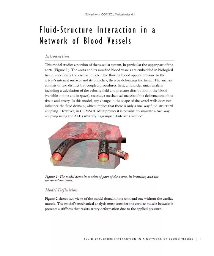
Solved with COMSOL Multiphysics 4.1 Fluid-Structure Interaction in a Network of Blood Vessels Introduction This model studies a portion of the vascular system, in particular the upper part of the aorta (Figure 1). The aorta and its ramified blood vessels are embedded in biological tissue, specifically the cardiac muscle. The flowing blood applies pressure to the artery’s internal surfaces and its branches, thereby deforming the tissue. The analysis consists of two distinct but coupled procedures: first, a fluid-dynamics analysis including a calculation of the velocity field and pressure distribution in the blood (variable in time and in space); second, a mechanical analysis of the deformation of the tissue and artery. In this model, any change in the shape of the vessel walls does not influence the fluid domain, which implies that there is only a one-way fluid-structural coupling. However, in COMSOL Multiphysics it is possible to simulate a two-way coupling using the ALE (arbitrary Lagrangian-Eulerian) method. Figure 1: The model domain consists of part of the aorta, its branches, and the surrounding tissue. Model Definition Figure 2 shows two views of the model domain, one with and one without the cardiac muscle. The model’s mechanical analysis must consider the cardiac muscle because it presents a stiffness that resists artery deformation due to the applied pressure. F L U I D - S T R U C T U R E I N T E R A C T I O N I N A N E T W O R K O F B L O O D VE S S E L S | 1
Solved with COMSOL Multiphysics 4.1 Figure 2: A view of the aorta and its ramification (branching vessels) with blood contained, shown both with (left) and without (right) the cardiac muscle. The main characteristics of the analyses are: •Fluid dynamics analysis Here the model solves the Navier-Stokes equations in the blood domain. At each surface where the model brings a vessel to an abrupt end, it represents the load with a known pressure distribution. •Mechanical analysis This analysis is nonlinear due to the assumption of a large displacement and the constitutive behavior of the materials (the model describes the response of the artery and cardiac muscle with an hyperelastic law similar to those for rubber components). Only the domains related to the biological tissues are active in this analysis. The model represents the load with the total stress distribution it computes during the fluid-dynamics analysis. AN A LY SI S O F R UBB ER -L IKE TI SS UE A ND A R T ER Y M ATE RI AL M OD E LS The analysis of rubber-like elastomers is generally a difficult task for several reasons: • The material can undergo very large strains (finite deformations). • The stress-strain relationship is generally nonlinear. • Many rubber-like materials are almost incompressible. You must revise standard displacement-based finite element formulations in order to arrive at correct results (mixed formulations). 2 | F L U I D - S T R U C T U R E I N T E R A C T I O N I N A N E T W O R K O F B L O O D VE S S E L S
Solved with COMSOL Multiphysics 4.1 You must pay particular attention to the definition of stress and strain measures. In a geometrically nonlinear analysis the assumptions about infinitesimal displacements are no longer valid. It is necessary to consider geometrical nonlinearity in a model when: • Significant rigid-body rotations occur (finite rotations). • The strains are no longer small (larger then a few percent). • The loading of the body depends on the deformation. All of these issues are dealt with in the hyperelastic material model built-in the Structural Mechanics Module. MATER IA LS The model in this example uses the following material properties: • Blood - density = 1060 kg/m3 - dynamic viscosity = 0.005 Ns/m2 • Artery - density = 960 kg/m3 - Neo-Hookean hyperelastic behavior: the coefficient equals 6.20·106 N/m2, while the bulk modulus equals 20 and corresponds to a value for Poisson’s ratio, , of 0.45. An equivalent elastic modulus equals 1.0·107 N/m2. - Cardiac muscle - density = 1200 kg/m3 - Neo-Hookean hyperelastic behavior: the coefficient equals 7.20·106 N/m2, while the bulk modulus equals 20 and corresponds to a value for Poisson’s ratio, , of 0.45. An equivalent elastic modulus equals 1.16·106 N/m2. F L U I D D Y N A M I C S A NA LY S I S The fluid dynamics analysis considers the solution of the 3D Navier-Stokes equations. You can do so in both a stationary case or in the time domain. To establish the F L U I D - S T R U C T U R E I N T E R A C T I O N I N A N E T W O R K O F B L O O D VE S S E L S | 3
Solved with COMSOL Multiphysics 4.1 boundary conditions, the model uses six pressure conditions with the configuration in Figure 3. P = Pressure 4. P 5. P 3. P 2. P 1. P 6. P Figure 3: Boundary conditions for the fluid-flow analysis. The pressure conditions are: • Section 1: 11,208 Pa • Section 2: 11,192 Pa • Section 3: 11,148 Pa • Section 4: 11,148 Pa • Section 5: 11,148 Pa • Section 6: 11,120 Pa For the time-dependent analysis, the model uses a simple trigonometric function to vary the pressure distribution over time: 1 2 t0 -- -s sin t f t (1) = 1 2 1 3 2 1 2 3 2 2 t cos -- -s -- -s -- - -- - -- - t – – 2 You implement this effect in COMSOL Multiphysics using a domain variable. 4 | F L U I D - S T R U C T U R E I N T E R A C T I O N I N A N E T W O R K O F B L O O D VE S S E L S
Solved with COMSOL Multiphysics 4.1 Results and Discussion First examine the steady flow field so as to compare its result to the transient case. Figure 4 shows a slice plot of the velocity field (that gives values in m/s). Figure 4: Velocity field color slice in the aorta and its ramification (branching). A final model accounts for the influence of large displacements and for the hyperelastic behavior of the biological tissues. Figure 5 shows the total displacement at the peak load (after 1 s). The displacements are in the order of 10 m, which suggests that the one-way multiphysics coupling is a reasonable approximation. F L U I D - S T R U C T U R E I N T E R A C T I O N I N A N E T W O R K O F B L O O D VE S S E L S | 5
Solved with COMSOL Multiphysics 4.1 Figure 5: Displacements in the blood vessel using a hyperelastic model. Notes About the COMSOL Implementation In this model, and many other cases, an analysis which is time dependent for one physics can be treated as quasi-static from the structural mechanics point of view. You can handle this by running the structural analysis as a parametric sweep over a number of static load cases, where the time is used as the parameter. This method is used here. Model Library path: Structural_Mechanics_Module/Bioengineering/ blood_vessel Modeling Instructions M OD EL W I Z A RD 1 Go to the Model Wizard window. 6 | F L U I D - S T R U C T U R E I N T E R A C T I O N I N A N E T W O R K O F B L O O D VE S S E L S
Solved with COMSOL Multiphysics 4.1 2 On the Select Space Dimension page, click Next to get a 3D geometry. 3 In the Add Physics tree, select Fluid Flow>Single-Phase Flow>Laminar Flow (spf). 4 Click Add Selected. 5 In the Add Physics tree, select Structural Mechanics>Solid Mechanics (solid). 6 Click Add Selected. 7 Click Next. 8 In the Studies tree, select Preset Studies for Selected Physics>Time Dependent. 9 Click Finish. GL O BA L D E FI N ITI O NS Parameters 1 In the Model Builder window, right-click Global Definitions and choose Parameters. 2 Go to the Settings window for Parameters. 3 Locate the Parameters section. In the Parameters table, enter the following settings: NAME EXPRESSION DESCRIPTION p01 11208[Pa] Pressure condition 1 p02 11192[Pa] Pressure condition 2 p03 11148[Pa] Pressure condition 3 p04 11148[Pa] Pressure condition 4 p05 11148[Pa] Pressure condition 5 p06 11120[Pa] Pressure condition 6 D EF IN I TIO N S Variables 1 1 In the Model Builder window, right-click Model 1>Definitions and choose Variables. 2 Go to the Settings window for Variables. 3 Locate the Variables section. In the Variables table, enter the following settings: NAME EXPRESSION (t<=0.5)*sin(pi*t[1/s])+(t>0.5)* (1.5-0.5*cos(-2*pi*(0.5-t[1/s]))) DESCRIPTION f Pressure distribution time dependence F L U I D - S T R U C T U R E I N T E R A C T I O N I N A N E T W O R K O F B L O O D VE S S E L S | 7
Solved with COMSOL Multiphysics 4.1 G EO M E T R Y 1 The geometry for this model is available as an MPHBIN-file. Import the geometry as follows. Import 1 1 In the Model Builder window, right-click Model 1>Geometry 1 and choose Import. 2 Go to the Settings window for Import. 3 Locate the Import section. Click the Browse button. 4 Browse to the model’s Model Library folder and double-click the file blood_vessel.mphbin. 5 Click the Import button. The length unit in the imported geometry is centimeters, while the default length unit in COMSOL Multiphysics is meters. Therefore, you need to rescale the geometry. Scale 1 1 In the Model Builder window, right-click Geometry 1 and choose Scale. 2 Go to the Settings window for Scale. 3 Locate the Scale Factor section. In the Factor edit field, type 0.01. 4 Select the object imp1 only. 5 Click the Build Selected button. 6 Click the Go to Default 3D View button on the Graphics toolbar. Form Union 1 In the Model Builder window, right-click Form Union and choose Build Selected. 8 | F L U I D - S T R U C T U R E I N T E R A C T I O N I N A N E T W O R K O F B L O O D VE S S E L S
Solved with COMSOL Multiphysics 4.1 2 Click the Transparency button on the Graphics toolbar to see the interior. D EF IN I TIO N S Next, define a number of selections as sets of geometric entities for use in setting up the model. Selection 1 1 In the Model Builder window, right-click Model 1>Definitions and choose Selection. 2 Select Domain 3 only. 3 Right-click Selection 1 and choose Rename. 4 Go to the Rename Selection dialog box and type blood in the New name edit field. 5 Click OK. Selection 2 1 Right-click Definitions and choose Selection. 2 Select Domain 2 only. 3 Right-click Selection 2 and choose Rename. 4 Go to the Rename Selection dialog box and type artery in the New name edit field. 5 Click OK. F L U I D - S T R U C T U R E I N T E R A C T I O N I N A N E T W O R K O F B L O O D VE S S E L S | 9
Solved with COMSOL Multiphysics 4.1 Selection 3 1 Right-click Definitions and choose Selection. 2 Select Domain 1 only. 3 Right-click Selection 3 and choose Rename. 4 Go to the Rename Selection dialog box and type muscle in the New name edit field. 5 Click OK. Selection 4 1 Right-click Definitions and choose Selection. 2 Go to the Settings window for Selection. 3 Locate the Geometric Scope section. From the Geometric entity level list, select Boundary. Select Boundary 38 only as follows: 4 Click Paste Selection, then go to the Paste Selection dialog box. 5 In the Selection edit field, type 38, then click OK to close the dialog box. 6 Right-click Selection 4 and choose Rename. 7 Go to the Rename Selection dialog box and type inlet in the New name edit field. 8 Click OK. Selection 5 1 Right-click Definitions and choose Selection. 2 Go to the Settings window for Selection. 3 Locate the Geometric Scope section. From the Geometric entity level list, select Boundary. 4 Select Boundary 19 only. 5 Right-click Selection 5 and choose Rename. 6 Go to the Rename Selection dialog box and type outlet1 in the New name edit field. 7 Click OK. Selection 6 1 Right-click Definitions and choose Selection. 2 Go to the Settings window for Selection. 3 Locate the Geometric Scope section. From the Geometric entity level list, select Boundary. 4 Select Boundary 9 only. 10 | F L U I D - S T R U C T U R E I N T E R A C T I O N I N A N E T W O R K O F B L O O D VE S S E L S
Solved with COMSOL Multiphysics 4.1 5 Right-click Selection 6 and choose Rename. 6 Go to the Rename Selection dialog box and type outlet2 in the New name edit field. 7 Click OK. Selection 7 1 Right-click Definitions and choose Selection. 2 Go to the Settings window for Selection. 3 Locate the Geometric Scope section. From the Geometric entity level list, select Boundary. 4 Select Boundary 41 only. 5 Right-click Selection 7 and choose Rename. 6 Go to the Rename Selection dialog box and type outlet3 in the New name edit field. 7 Click OK. Selection 8 1 Right-click Definitions and choose Selection. 2 Go to the Settings window for Selection. 3 Locate the Geometric Scope section. From the Geometric entity level list, select Boundary. 4 Select Boundary 70 only. 5 Right-click Selection 8 and choose Rename. 6 Go to the Rename Selection dialog box and type outlet4 in the New name edit field. 7 Click OK. Selection 9 1 Right-click Definitions and choose Selection. 2 Go to the Settings window for Selection. 3 Locate the Geometric Scope section. From the Geometric entity level list, select Boundary. 4 Select Boundary 86 only. 5 Right-click Selection 9 and choose Rename. 6 Go to the Rename Selection dialog box and type outlet5 in the New name edit field. 7 Click OK. Selection 10 1 Right-click Definitions and choose Selection. F L U I D - S T R U C T U R E I N T E R A C T I O N I N A N E T W O R K O F B L O O D VE S S E L S | 11
Solved with COMSOL Multiphysics 4.1 2 Go to the Settings window for Selection. 3 Locate the Geometric Scope section. From the Geometric entity level list, select Boundary. 4 Select Boundaries 1–6, 12, 26, 27, 30, 33, 64, 67, 85, and 87 only. 5 Right-click Selection 10 and choose Rename. 6 Go to the Rename Selection dialog box and type roller boundaries in the New name edit field. 7 Click OK. The roller boundaries are the free boundaries of muscle and artery that are neither in contact with each other nor with blood. Selection 11 1 Right-click Definitions and choose Selection. 2 Go to the Settings window for Selection. 3 Locate the Geometric Scope section. From the Geometric entity level list, select Boundary. 4 Select the All boundaries check box. 5 Select Boundaries 10, 11, 16, 17, 20, 21, 23, 24, 36, 37, 39, 40, 42, 43, 45, 46, 50–53, 58, 59, 61, 62, 68, 69, 71, 72, 75, 76, 79, 80, 82, and 83 only. 6 Right-click Selection 11 and choose Rename. 7 Go to the Rename Selection dialog box and type loaded boundaries in the New name edit field. 8 Click OK. The loaded boundaries are the inner boundaries of the artery that are in contact with blood. Selection 12 1 Right-click Definitions and choose Selection. 2 Select Domain 2 only. 3 Go to the Settings window for Selection. 4 Locate the Geometric Scope section. From the Selection output list, select Adjacent boundaries. 5 Select the Interior boundaries check box. 6 Right-click Selection 12 and choose Rename. 12 | F L U I D - S T R U C T U R E I N T E R A C T I O N I N A N E T W O R K O F B L O O D VE S S E L S
Solved with COMSOL Multiphysics 4.1 7 Go to the Rename Selection dialog box and type artery walls in the New name edit field. 8 Click OK. LA MI N AR F LOW 1 In the Model Builder window, click Model 1>Laminar Flow. 2 Go to the Settings window for Laminar Flow. 3 Locate the Domains section. From the Selection list, select blood. 4 Locate the Physical Model section. From the Compressibility list, select Incompressible flow. Inlet 1 1 Right-click Model 1>Laminar Flow and choose Inlet. 2 Go to the Settings window for Inlet. 3 Locate the Boundaries section. From the Selection list, select inlet. 4 Locate the Boundary Condition section. From the Boundary condition list, select Pressure, no viscous stress. 5 In the p0 edit field, type p01*f. Outlet 1 1 In the Model Builder window, right-click Laminar Flow and choose Outlet. 2 Go to the Settings window for Outlet. 3 Locate the Boundaries section. From the Selection list, select outlet1. 4 Locate the Boundary Condition section. In the p0 edit field, type p02*f. Outlet 2 1 In the Model Builder window, right-click Laminar Flow and choose Outlet. 2 Go to the Settings window for Outlet. 3 Locate the Boundaries section. From the Selection list, select outlet2. 4 Locate the Boundary Condition section. In the p0 edit field, type p03*f. Outlet 3 1 In the Model Builder window, right-click Laminar Flow and choose Outlet. 2 Go to the Settings window for Outlet. 3 Locate the Boundaries section. From the Selection list, select outlet3. 4 Locate the Boundary Condition section. In the p0 edit field, type p04*f. F L U I D - S T R U C T U R E I N T E R A C T I O N I N A N E T W O R K O F B L O O D VE S S E L S | 13
Solved with COMSOL Multiphysics 4.1 Outlet 4 1 In the Model Builder window, right-click Laminar Flow and choose Outlet. 2 Go to the Settings window for Outlet. 3 Locate the Boundaries section. From the Selection list, select outlet4. 4 Locate the Boundary Condition section. In the p0 edit field, type p05*f. Outlet 5 1 In the Model Builder window, right-click Laminar Flow and choose Outlet. 2 Go to the Settings window for Outlet. 3 Locate the Boundaries section. From the Selection list, select outlet5. 4 Locate the Boundary Condition section. In the p0 edit field, type p06*f. S O L ID M E C H A N I C S 1 In the Model Builder window, click Model 1>Solid Mechanics. 2 Select Domains 1 and 2 only. 3 Go to the Settings window for Solid Mechanics. 4 Click to expand the Discretization section. 5 From the Displacement field list, select Linear. This matches the default order of the temperature field elements. Hyperelastic Material Model 1 1 Right-click Model 1>Solid Mechanics and choose Hyperelastic Material Model. 2 Go to the Settings window for Hyperelastic Material Model. 3 Locate the Domains section. From the Selection list, select artery. Hyperelastic Material Model 2 1 In the Model Builder window, right-click Solid Mechanics and choose Hyperelastic Material Model. 2 Go to the Settings window for Hyperelastic Material Model. 3 Locate the Domains section. From the Selection list, select muscle. Roller 1 1 In the Model Builder window, right-click Solid Mechanics and choose Roller. 2 Go to the Settings window for Roller. 3 Locate the Boundaries section. From the Selection list, select roller boundaries. 14 | F L U I D - S T R U C T U R E I N T E R A C T I O N I N A N E T W O R K O F B L O O D VE S S E L S
Solved with COMSOL Multiphysics 4.1 Boundary Load 1 1 In the Model Builder window, right-click Solid Mechanics and choose Boundary Load. 2 Go to the Settings window for Boundary Load. 3 Locate the Boundaries section. From the Selection list, select loaded boundaries. 4 Locate the Force section. Specify the FA vector as -spf.T_stressx x -spf.T_stressy y -spf.T_stressz z MATER IA LS Material 1 1 In the Model Builder window, right-click Model 1>Materials and choose Material. 2 Go to the Settings window for Material. 3 Locate the Geometric Scope section. From the Selection list, select blood. 4 Locate the Material Contents section. In the Material Contents table, enter the following settings: PROPERTY Density NAME rho VALUE 1060 0.005 Dynamic viscosity mu 5 Right-click Material 1 and choose Rename. 6 Go to the Rename Material dialog box and type blood in the New name edit field. 7 Click OK. Material 2 1 Right-click Materials and choose Material. 2 Go to the Settings window for Material. 3 Locate the Geometric Scope section. From the Selection list, select artery. 4 Locate the Material Contents section. In the Material Contents table, enter the following settings: PROPERTY Lamé constant NAME lambda VALUE 20*mu-2*mu/3 F L U I D - S T R U C T U R E I N T E R A C T I O N I N A N E T W O R K O F B L O O D VE S S E L S | 15
Solved with COMSOL Multiphysics 4.1 PROPERTY NAME VALUE 6.20e6 Lamé constant mu 960 Density rho 5 Right-click Material 2 and choose Rename. 6 Go to the Rename Material dialog box and type artery in the New name edit field. 7 Click OK. Material 3 1 Right-click Materials and choose Material. 2 Go to the Settings window for Material. 3 Locate the Geometric Scope section. From the Selection list, select muscle. 4 Locate the Material Contents section. In the Material Contents table, enter the following settings: PROPERTY Lamé constant NAME lambda VALUE 20*mu-2*mu/3 7.20e6 Lamé constant mu 1200 Density rho 5 Right-click Material 3 and choose Rename. 6 Go to the Rename Material dialog box and type muscle in the New name edit field. 7 Click OK. M ES H 1 Free Tetrahedral 1 In the Model Builder window, right-click Model 1>Mesh 1 and choose Free Tetrahedral. Size 1 1 In the Model Builder window, right-click Free Tetrahedral 1 and choose Size. 2 Go to the Settings window for Size. 3 Locate the Geometric Scope section. From the Geometric entity level list, select Domain. 4 From the Selection list, select blood. 5 Locate the Element Size section. Click the Custom button. 6 Click to expand the Element Size Parameters section. 16 | F L U I D - S T R U C T U R E I N T E R A C T I O N I N A N E T W O R K O F B L O O D VE S S E L S
Solved with COMSOL Multiphysics 4.1 7 Select the Maximum element size check box. 8 In the associated edit field, type 1e-3. Size 1 In the Model Builder window, click Size. 2 Go to the Settings window for Size. 3 Locate the Element Size section. From the Predefined list, select Fine. 4 Click the Build All button. S T U D Y 1 The structural problem is quasi-static, so you can use the time just as a parameter for the parametric solver, together with a stationary solver. Thus the whole study can be divided into two steps. First run the transient study for the fluid-mechanics part of the problem and then use the stationary solver to solve the structural part using the solution from first transient study. Step 1: Time Dependent 1 In the Model Builder window, expand the Study 1 node, then click Step 1: Time Dependent. 2 Go to the Settings window for Time Dependent. F L U I D - S T R U C T U R E I N T E R A C T I O N I N A N E T W O R K O F B L O O D VE S S E L S | 17
Solved with COMSOL Multiphysics 4.1 3 Locate the Study Settings section. In the Times edit field, type range(0,0.05,1). 4 Locate the Physics Selection section. In the Physics interfaces list, select Solid mechanics (solid). 5 Clear the Use in this study check box. 6 In the Model Builder window, right-click Study 1 and choose Compute. R E S U L TS By default, you get a surface and a slice plot of the velocity field. Modify the slice plot in the second plot group to reproduce the plot in Figure 4. 3D Plot Group 2 1 Click the Transparency button on the Graphics toolbar to restore the original transparency state. 2 In the Model Builder window, expand the Results>3D Plot Group 2 node, then click Slice 1. 3 Go to the Settings window for Slice. 4 Locate the Plane Data section. From the Plane list, select zx-planes. 5 In the Planes edit field, type 1. 6 Click the Plot button. 7 Click the Go to Default 3D View button on the Graphics toolbar. Now turn to the structural problem. G LO B AL D EF IN I TIO N S Parameters 1 In the Model Builder window, click Global Definitions>Parameters. 2 Go to the Settings window for Parameters. 3 Locate the Parameters section. In the Parameters table, enter the following settings: NAME EXPRESSION DESCRIPTION t 0 Time as parameter M OD EL W I Z A RD 1 In the Model Builder window, right-click the root node and choose Add Study. 2 Go to the Model Wizard window. 3 In the Studies tree, select Preset Studies for Selected Physics>Stationary. 18 | F L U I D - S T R U C T U R E I N T E R A C T I O N I N A N E T W O R K O F B L O O D VE S S E L S
Solved with COMSOL Multiphysics 4.1 4 Click Finish. S T U D Y 2 Step 1: Stationary 1 In the Model Builder window, click Study 2>Step 1: Stationary. 2 Go to the Settings window for Stationary. 3 Locate the Physics Selection section. 4 In the Physics interfaces list, select Laminar flow (spf). 5 Clear the Use in this study check box. Parametric Sweep 1 In the Model Builder window, right-click Study 2 and choose Parametric Sweep. 2 Go to the Settings window for Parametric Sweep. 3 Locate the Study Settings section. Under Parameter names, click Add. 4 Go to the Add dialog box. 5 In the Parameter names list, select Time as parameter (t). 6 Click the OK button. 7 Go to the Settings window for Parametric Sweep. 8 Locate the Study Settings section. In the Parameter values edit field, type range(0,0.05,1). Solver 2 1 In the Model Builder window, right-click Study 2 and choose Show Default Solver. 2 In the Model Builder window, expand the Study 2>Solver Configurations>Solver 2>Dependent Variables 1 node, then click Dependent Variables 1. 3 Go to the Settings window for Dependent Variables. 4 Locate the Values of Variables Not Solved For section. From the Method list, select Solution. 5 From the Solution list, select Solver 1. 6 From the Time list, select All. 7 In the Model Builder window, click Dependent Variables 1>mod1_u2. 8 Go to the Settings window for Field. 9 Locate the Scaling section. From the Method list, select Manual. 1 0 In the Scale edit field, type 1e-5. F L U I D - S T R U C T U R E I N T E R A C T I O N I N A N E T W O R K O F B L O O D VE S S E L S | 19
Solved with COMSOL Multiphysics 4.1 11 In the Model Builder window, right-click Study 2 and choose Compute. R E S U L TS To reproduce the plot shown in Figure 5, begin by defining a selection for the solution data set to make interior boundaries visible in the plot. Data Sets 1 In the Model Builder window, expand the Results>Data Sets node. 2 Right-click Solution 2 and choose Add Selection. 3 Go to the Settings window for Selection. 4 Locate the Geometric Scope section. From the Geometric entity level list, select Boundary. 5 From the Selection list, select artery walls. 3D Plot Group 3 1 In the Model Builder window, expand the 3D Plot Group 3 node, then click Surface 1. 2 Go to the Settings window for Surface. 3 In the upper-right corner of the Expression section, click Replace Expression. 4 From the menu, choose Solid Mechanics>Total displacement (solid.disp). 5 Locate the Expression section. From the Unit list, select µm. 6 Click the Plot button. 7 Right-click Surface 1 and choose Deformation. 8 Go to the Settings window for Deformation. 9 In the upper-right corner of the Expression section, click Replace Expression. 10 From the menu, choose Solid Mechanics>Displacement field (u2, v2, w2). 11 Locate the Scale section. Select the Scale factor check box. 12 In the associated edit field, type 300. 13 In the Model Builder window, click 3D Plot Group 3. 14 Go to the Settings window for 3D Plot Group. 15 Locate the Plot Settings section. Select the Title check box. 16 In the associated edit field, type Time=1 Surface: Total displacement (µm) Surface Deformation: Displacement field. 17 Click the Plot button. 18 Click the Go to Default 3D View button on the Graphics toolbar. 20 | F L U I D - S T R U C T U R E I N T E R A C T I O N I N A N E T W O R K O F B L O O D VE S S E L S