Download
1 / 47
470 likes | 779 Views
Algorithmic Analysis. Analysis of Algorithms. Input. Algorithm. Output. An algorithm is a step-by-step procedure for solving a problem in a finite amount of time. Algorithm Analysis. Foundations of Algorithm Analysis and Data Structures. Analysis:

E N D
Analysis of Algorithms Input Algorithm Output An algorithm is a step-by-step procedure for solving a problem in a finite amount of time.
Algorithm Analysis • Foundations of Algorithm Analysis and Data Structures. • Analysis: • How to predict an algorithm’s performance • How well an algorithm scales up • How to compare different algorithms for a problem • Data Structures • How to efficiently store, access, manage data • Data structures effect algorithm’s performance
Example Algorithms • Two algorithms for computing the Factorial • Which one is better? • int factorial (int n) { if (n <= 1) return 1; else return n * factorial(n-1); } • int factorial (int n) { if (n<=1) return 1; else { fact = 1; for (k=2; k<=n; k++) fact *= k; return fact; } }
Examples of famous algorithms • Constructions of Euclid • Newton's root finding • Fast Fourier Transform • Compression (Huffman, Lempel-Ziv, GIF, MPEG) • DES, RSA encryption • Simplex algorithm for linear programming • Shortest Path Algorithms (Dijkstra, Bellman-Ford) • Error correcting codes (CDs, DVDs) • TCP congestion control, IP routing • Pattern matching • Delaunay Triangulation
Why Efficient Algorithms Matter • Suppose N = 106 • A PC can read/process N records in 1 sec. • But if some algorithm does N*N computation, then it takes 1M seconds = 11 days!!! • 100 City Traveling Salesman Problem. • A supercomputer checking 100 billion tours/sec still requires 10100years! • Fast factoring algorithms can break encryption schemes. Algorithms research determines what is safe code length. (> 100 digits)
How to Measure Algorithm Performance • What metric should be used to judge algorithms? • Length of the program (lines of code) • Ease of programming (bugs, maintenance) • Memory required • Running time • Running time is the dominant standard. • Quantifiable and easy to compare • Often the critical bottleneck
Abstraction • An algorithm may run differently depending on: • the hardware platform (PC, Cray, Sun) • the programming language (C, Java, C++) • the programmer (you, me, Bill Joy) • While different in detail, all hardware and prog models are equivalent in some sense: Turing machines. • It suffices to count basic operations. • Crude but valuable measure of algorithm’s performance as a function of input size.
Average, Best, and Worst-Case • On which input instances should the algorithm’s performance be judged? • Average case: • Real world distributions difficult to predict • Best case: • Seems unrealistic • Worst case: • Gives an absolute guarantee • We will use the worst-case measure.
Average Case vs. Worst Case Running Timeof an algorithm • An algorithm may run faster on certain data sets than on others. • Finding the average case can be very difficult, so typically algorithms are measured by the worst-case time complexity. • Also, in certain application domains (e.g., air traffic control, surgery, IP lookup) knowing the worst-case time complexity is of crucial importance.
Examples • Vector addition Z = A+B for (int i=0; i<n; i++) Z[i] = A[i] + B[i]; T(n) = c n • Vector (inner) multiplication z =A*B z = 0; for (int i=0; i<n; i++) z = z + A[i]*B[i]; T(n) = c’ + c1 n
Examples • Vector (outer) multiplication Z = A*BT for (int i=0; i<n; i++) for (int j=0; j<n; j++) Z[i,j] = A[i] * B[j]; T(n) = c2 n2; • A program does all the above T(n) = c0 + c1 n + c2 n2;
Simplifying the Bound • T(n) = ck nk + ck-1 nk-1 + ck-2 nk-2 + … + c1 n + co • too complicated • too many terms • Difficult to compare two expressions, each with 10 or 20 terms • Do we really need that many terms?
Simplifications • Keep just one term! • the fastest growing term (dominates the runtime) • No constant coefficients are kept • Constant coefficients affected by machines, languages, etc. • Asymtotic behavior (as n gets large) is determined entirely by the leading term. • Example. T(n) = 10 n3 + n2 + 40n + 800 • If n = 1,000, then T(n) = 10,001,040,800 • error is 0.01% if we drop all but the n3 term • In an assembly line the slowest worker determines the throughput rate
Simplification • Drop the constant coefficient • Does not effect the relative order
Simplification • The faster growing term (such as 2n) eventually will outgrow the slower growing terms (e.g., 1000 n) no matter what their coefficients! • Put another way, given a certain increase in allocated time, a higher order algorithm will not reap the benefit by solving much larger problem
Complexity and Tractability Assume the computer does 1 billion ops per sec.
2n n2 2n n2 n3 n log n n n3 n log n log n n log n
Another View • More resources (time and/or processing power) translate into large problems solved if complexity is low
Asympotics • They all have the same “growth” rate
Caveats • Follow the spirit, not the letter • a 100n algorithm is more expensive than n2 algorithm when n < 100 • Other considerations: • a program used only a few times • a program run on small data sets • ease of coding, porting, maintenance • memory requirements
Asymptotic Notations • Big-O, “bounded above by”: T(n) = O(f(n)) • For some c and N, T(n) c·f(n) whenever n > N. • Big-Omega, “bounded below by”: T(n) = W(f(n)) • For some c>0 and N, T(n) c·f(n) whenever n > N. • Same as f(n) = O(T(n)). • Big-Theta, “bounded above and below”: T(n) = Q(f(n)) • T(n) = O(f(n)) and also T(n) = W(f(n)) • Little-o, “strictly bounded above”: T(n) = o(f(n)) • T(n)/f(n) 0 as n
By Pictures • Big-Oh (most commonly used) • bounded above • Big-Omega • bounded below • Big-Theta • exactly • Small-o • not as expensive as ...
Summary (Why O(n)?) • T(n) = ck nk + ck-1 nk-1 + ck-2 nk-2 + … + c1 n + co • Too complicated • O(nk ) • a single term with constant coefficient dropped • Much simpler, extra terms and coefficients do not matter asymptotically • Other criteria hard to quantify
Runtime Analysis • Useful rules • simple statements (read, write, assign) • O(1) (constant) • simple operations (+ - * / == > >= < <= • O(1) • sequence of simple statements/operations • rule of sums • for, do, while loops • rules of products
Runtime Analysis (cont.) • Two important rules • Rule of sums • if you do a number of operations in sequence, the runtime is dominated by the most expensive operation • Rule of products • if you repeat an operation a number of times, the total runtime is the runtime of the operation multiplied by the iteration count
Runtime Analysis (cont.) if (cond) then O(1) body1T1(n) else body2T2(n) endif T(n) = O(max (T1(n), T2(n))
Runtime Analysis (cont.) • Method calls • A calls B • B calls C • etc. • A sequence of operations when call sequences are flattened T(n) = max(TA(n), TB(n), TC(n))
Example for (i=1; i<n; i++) if A(i) > maxVal then maxVal= A(i); maxPos= i; Asymptotic Complexity: O(n)
Example for (i=1; i<n-1; i++) for (j=n; j>= i+1; j--) if (A(j-1) > A(j)) then temp = A(j-1); A(j-1) = A(j); A(j) = tmp; endif endfor endfor • Asymptotic Complexity is O(n2)
Max Subsequence Problem • Given a sequence of integers A1, A2, …, An, find the maximum possible value of a subsequence Ai, …, Aj. • Numbers can be negative. • You want a contiguous chunk with largest sum. • Example: -2, 11, -4, 13, -5, -2 • The answer is 20 (subseq. A2 through A4). • We will discuss 4 different algorithms, with time complexities O(n3), O(n2), O(n log n), and O(n). • With n = 106, algorithm 1 won’t finish in our lifetime; algorithm 4 will take a fraction of a second!
Algorithm 1 for Max Subsequence Sum • Given A1,…,An , find the maximum value of Ai+Ai+1+···+Aj 0 if the max value is negative int maxSum = 0; for( int i = 0; i < a.size( ); i++ ) for( int j = i; j < a.size( ); j++ ) { int thisSum = 0; for( int k = i; k <= j; k++ ) thisSum += a[ k ]; if( thisSum > maxSum ) maxSum = thisSum; } return maxSum; • Time complexity: O(n3)
Algorithm 2 • Idea: Given sum from i to j-1, we can compute the sum from i to j in constant time. • This eliminates one nested loop, and reduces the running time to O(n2). into maxSum = 0; for( int i = 0; i < a.size( ); i++ ) int thisSum = 0; for( int j = i; j < a.size( ); j++ ) { thisSum += a[ j ]; if( thisSum > maxSum ) maxSum = thisSum; } return maxSum;
Algorithm 3 • This algorithm uses divide-and-conquer paradigm. • Suppose we split the input sequence at midpoint. • The max subsequence is entirely in the left half, entirely in the right half, or it straddles the midpoint. • Example: left half | right half 4 -3 5 -2 | -1 2 6 -2 • Max in left is 6 (A1 through A3); max in right is 8 (A6 through A7). But straddling max is 11 (A1 thru A7).
Algorithm 3 (cont.) • Example: left half | right half 4 -3 5 -2 | -1 2 6 -2 • Max subsequences in each half found by recursion. • How do we find the straddling max subsequence? • Key Observation: • Left half of the straddling sequence is the max subsequence beginning with -2! • Right half is the max subsequence beginning with -1! • A linear scan lets us compute these in O(n) time.
Algorithm 3: Analysis • The divide and conquer is best analyzed through recurrence: T(1) = 1 T(n) = 2T(n/2) + O(n) • This recurrence solves to T(n) = O(n log n).
Algorithm 4 • Time complexity clearly O(n) • But why does it work? I.e. proof of correctness. 2, 3, -2, 1, -5, 4, 1, -3, 4, -1, 2 int maxSum = 0, thisSum = 0; for( int j = 0; j < a.size( ); j++ ) { thisSum += a[ j ]; if ( thisSum > maxSum ) maxSum = thisSum; else if ( thisSum < 0 ) thisSum = 0; } return maxSum; }
Proof of Correctness • Max subsequence cannot start or end at a negative Ai. • More generally, the max subsequence cannot have a prefix with a negative sum. Ex: -2 11 -4 13 -5 -2 • Thus, if we ever find that Ai through Aj sums to < 0, then we can advance i to j+1 • Proof. Suppose j is the first index after i when the sum becomes < 0 • The max subsequence cannot start at any p between i and j. Because Ai through Ap-1 is positive, so starting at i would have been even better.
Algorithm 4 int maxSum = 0, thisSum = 0; for( int j = 0; j < a.size( ); j++ ) { thisSum += a[ j ]; if ( thisSum > maxSum ) maxSum = thisSum; else if ( thisSum < 0 ) thisSum = 0; } return maxSum • The algorithm resets whenever prefix is < 0. Otherwise, it forms new sums and updates maxSum in one pass.
Run Time for Recursive Programs • T(n) is defined recursively in terms of T(k), k<n • The recurrence relations allow T(n) to be “unwound” recursively into some base cases (e.g., T(0) or T(1)). • Examples: • Factorial • Hanoi towers
Example: Factorial int factorial (int n) { if (n<=1) return 1; else return n * factorial(n-1); } factorial (n) = n*n-1*n-2* … *1 n * factorial(n-1) n-1 * factorial(n-2) n-2 * factorial(n-3) … 2 *factorial(1) T(n) T(n-1) T(n-2) T(1)
Example: Factorial (cont.) int factorial1(int n) { if (n<=1) return 1; else { fact = 1; for (k=2;k<=n;k++) fact *= k; return fact; } } • Both algorithms are O(n). • An illustration that two algorithms may have the same order, but will run at different speed on real computers
Example: Hanoi Towers • Hanoi(n,A,B,C) = • Hanoi(n-1,A,C,B)+Hanoi(1,A,B,C)+Hanoi(n-1,C,B,A)
Worst Case, Best Case, and Average Case template<class T> void SelectionSort(T a[], int n) { for (int size=n; (size>1); size--) { int pos = 0; // find largest for (int i = 1; i < size; i++) if (a[pos] <= a[i]) pos = i; Swap(a[pos], a[size - 1]); } } // Early-terminating version of selection sort bool sorted = false; !sorted && sorted = true; else sorted = false;// out of order • Worst Case • Best Case
c f(N) T(N) n0 f(N) • T(N)=6N+4 : n0=4 and c=7, f(N)=N • T(N)=6N+4 <= c f(N) = 7N for N>=4 • 7N+4 = O(N) • 15N+20 = O(N) • N2=O(N)? • N log N = O(N)? • N log N = O(N2)? • N2 = O(N log N)? • N10 = O(2N)? • 6N + 4 = W(N) ? 7N? N+4 ? N2? N log N? • N log N = W(N2)? • 3 = O(1) • 1000000=O(1) • Sum i = O(N)? T(N)=O(f(N))