Download
1 / 19
220 likes | 528 Views
Conditional & Joint Probability. A brief digression back to joint probability: i.e. both events O and H occur. Again, we can express joint probability in terms of their separate conditional and unconditional probabilities. This key result turns out to be exceedingly useful!.

E N D
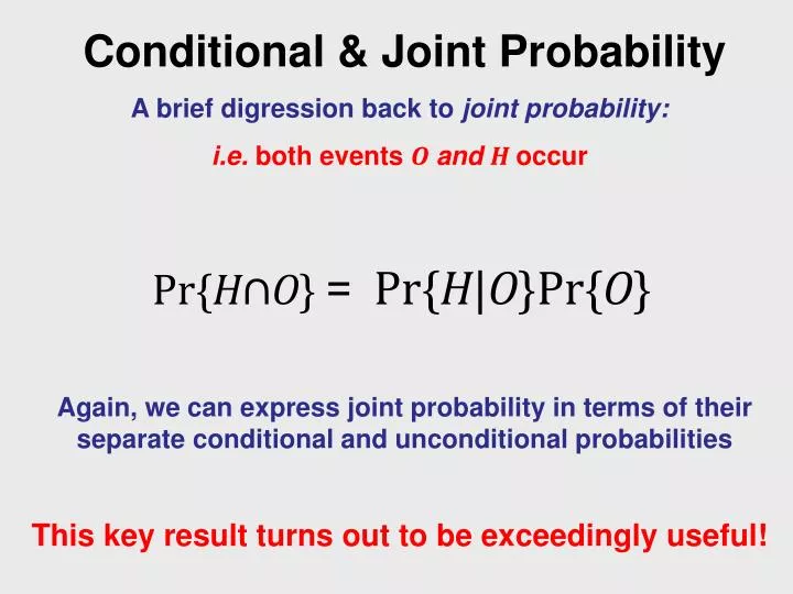
Conditional & Joint Probability A brief digression back to joint probability: i.e. both events OandH occur Again, we can express joint probability in terms of their separate conditional and unconditional probabilities This key result turns out to be exceedingly useful!
Conditional Probability Converting expressions of joint probability We can therefore express everything only in terms of reciprocal conditional and unconditional probabilities: The intersection operator makes no assertion regarding order: This is usually expressed in a slightly rearranged form…
Conditional Probability Bayes’ theorem expresses the essence of inference We can think of this as allowing us to compute the probability of some hidden event H given that some observable event O has occurred, provided we know the probability of the observed event Oassuming that hidden event H has occurred Bayes’ theorem is a recipe for problems involving conditional probability
Conditional Probability Normalizing the probabilities For convenience, we often replace the probability of the observed event O with the sum over all possible values of H of the joint probabilities of O and H. Whew! But consider that if we now calculated Pr{H|O} for every H, the sum of these would be one, which is just as a probability should behave… This summing of the expression in numerator “normalizes” the probabilities
Conditional Probability Bayes’ theorem as a recipe for inference The observable probability Generally, care must be taken to ensure that our observables have no uncertainty, otherwise they are really hidden!!! The prior Our best guess about H before any observation is made. Often we will makeneutral assumptions, resulting in an uninformative prior. But priors can also come from the posterior results from some earlier experiment. How best to choose priors is an essential element of Bayesian analysis The likelihood model We’ve seen already that the probability of an observation given a hidden parameter is really a likelihood. Choosing a likelihood model is akin to proposing some process, H, by which the observation, O, might have come about The posterior Think of this perhaps as the evidence for some specific model H given the set of observations O. We are making an inference about H on the basis of O Bayes’ theorem is so important that each part of this recipe has a special name
The Backward Algorithm Many paths give rise to the same sequence X We would often like to know the total probability of some sequence: But wait! Didn’t we already solve this problem using the forward algorithm!? Well, yes, but we’re going to solve it again by iterating backwards through the sequence instead of forwards P(x) = Sometimes, the trip isn’t about the destination. Stick with me!
The Backward Algorithm Defining the backward variable “The backward variable for state k at position i” bk(i) = P(xi+1 … xL|pi = k) “the probability of the sequence from the end to the symbol at position i, given that the path at position i is k” Since we are effectively stepping “backwards” through the event sequence, this is formulated as a statement of conditional probability rather than in terms of joint probability as are forward variables
The Backward Algorithm What if we had in our possession all of the backward variables for 1, the first position of the sequence? To get the overall probability of the sequence, we would need only sum the backward variables for each state (after correcting for the probability of the initial transition from Start) P(X) = We’ll obtain these “initial position” backward variables in a manner directly analogous to the method in the forward algorithm…
The Backward Algorithm A recursive definition for backward variables bk(i) = P(xi+1 … xL|pi = k) As always with a dynamic programming algorithm, we recursively define the variables.. But this time in terms of their own values at later positions in the sequence… The termination condition is satisfied and the basis case provided by virtue of the fact that sequences are finite and in this case we must eventually (albeit implicitly) come to the End state bk(i-1) =
The Backward Algorithm If you understand forward, you already understand backward! Initialization: bk(L) = 1 for all states k Recursion (i = L-1,…,1): bk(i) = el(xi + 1) · bl(i +1) · Termination: P(X) = We usually don’t need the termination step, except to check that the result is the same as from forward… So why bother with the backward algorithm in the first place?
The Backward Algorithm The probability of a sequence summed across all possible state paths S 0.1 0.9 A: 0.30 A: 0.20 0.5 C: 0.35 C: 0.25 G: 0.15 G: 0.25 T: 0.20 T: 0.30 0.5 0.4 0.6 State “+” State “-” _ A C G P(x) = 0.5 * 0.25 * 0.2 0.5 * 0.15 * 1 End 1 0.5 * 0.35 * 0.19 0.5 * 0.25 * 1 S =0.05825 S= 0.2 0.2 0.1 * 0.3 * 0.05825 0.9 * 0.2 * 0.0566 S= 0.0119355 0.6 * 0.25 * 0.2 0.6 * 0.15 * 1 1 0.4 * 0.25 * 1 0.4 * 0.35 * 0.19 0.0119355 S = 0.0566 S= 0.19 The backward algorithm takes its name from its backwards iteration through the sequence
The Decoding Problem The most probable state path The Viterbi algorithm will calculate the most probable state path, thereby allowing us to “decode” the state path in cases where the true state path is hidden _64622311445316146343245452316262524425613233524355442454134246666215124646526536662616666426446665162436615266416215651 SFFFFFFFFFFFFFLLLLFFFFFFFFFFFFFFFFFFFFFFFFFFFFFFFFFFFFFFFFFLLLLLLLLLLLLLLLLLLLLLLLLLLLLLLLLLLLLLLLLLLLLLLLLLLLLFFFFFFFFF SFFFFFFFFFFFFFFFFFFFFFFFFFFFFFFFFFFFFFFFFFFFFFFFFFFFFFFFFFFFFFLLLLLLLLLLLLLLLLLLLLLLLLLLLLLLLLLLLLLLLLLLLLLLLLLLLLLLLLLL Sequence True state path Viterbi patha.k.aMPSP p*= argmax P(x, p |θ) p*= argmax P(x, p) p p The Viterbi algorithm generally does a good job of recovering the state path…
The Decoding Problem Limitations of the most probable state path …but the most probable state path might not always be the best choice for further inference on the sequence • There may be other paths, sometimes several, that result in probabilities nearly as good as the MPSP • The MPSP tells us about the probability of the entire path, but it doesn’t actually tell us what the most probable state might be for some particular observation xi • More specifically, we might want to know: “the probability that observation xiresulted from being in state k, given the observed sequence x” P(pi = k|x) This is the posterior probabilityof state k at position i when sequence x is known
Calculating the Posterior Probabilities The approach is a little bit indirect…. We can sometimes ask a slightly different or related question, and see if that gets us closer to the result we seek Maybe we can first say something about the probability of producing the entire observed sequence with observation xi resulting from having been in state k….. = P(x,pi = k) P(x1…xi, pi = k)·P(xi+1…xL|x1…xi, pi = k) = P(x1…xi, pi = k)·P(xi+1…xL|pi = k) Does anything here look like something we may have seen before??
Calculating the Posterior Probabilities Limitations of the most probable state path P(x,pi = k) = P(x1…xi, pi = k)·P(xi+1…xL|pi = k) = fk(i)·bk(i) These terms are exactly our now familiar forward and backward variables!
Calculating the Posterior Probabilities Putting it all together using Baye’s theorem fk(i)·bk(i) P(pi = k|x) = P(x|pi = k)·P(pi = k) P(x,pi = k) P(x) Remember, we can get P(x) directly from either the forward or backward algorithm! We now have all of the necessary ingredients required to apply Baye’s theorem… We can now therefore find the posterior probability of being in state k for each position i in the sequence! We need only run both the forward and the backward algorithms to generate the values we need. Python: we probably want to store our forward and backward values as instance variables rather than method variables OK, but what can we really do with these posterior probabilities?
Posterior Decoding Making use of the posterior probabilities Two primary applications of the posterior state path probabilities • We can define an alternative state path to the most probable state path: ˰ pi = argmax P(pi = k | x) k This alternative to Viterbi decoding is most useful when we are most interested in the what the state might be at some particular point or points. It’s possible that the overall path suggested by this might not be particularly likely In some scenarios, the overall path might not even be a permitted path through the model!
Posterior Decoding Plotting the posterior probabilities Key:true path /Viterbi path / posterior path _44263143366636346665525516166566666224264513226235262443416 SFFFFFFFFLLLLLLLLLLLFFLLLLLFFLLLLLLLLFFFFFFFFFFFFFFFFFFFLLLL SFFFFFFFFFLLLLLLLLLLLLLLLLLLLLLLLLLLFFFFFFFFFFFFFFFFFFFFFFFF FFFFFFFFFLLLLLLLLLLLLFFFFLLLLLLLLLLLLFFFFFFFFFFFFFFFFFFFFFFF myHMM.generate(60,143456789) Since we know individual probabilities at each position we can easily plot the posterior probabilities
Posterior Decoding Plotting the posterior probabilities with matplotlib Assuming that we have list variables self._x containing the range of the sequence and self._y containing the posterior probabilities… from pylab import * # this line at the beginning of the file . . . class HMM(object): . . . # all your other stuff defshow_posterior(self): if self._x and self._y: plot (self._x, self._y) show() return Note: you may need to convert the log_float probabilities back to normal floats I found it more convenient to just define the __float__() method in log_float