Download
1 / 103
1.04k likes | 1.25k Views
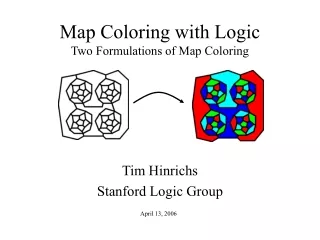
Map Coloring with Logic Two Formulations of Map Coloring. Tim Hinrichs Stanford Logic Group. Map Coloring. Map Coloring. Color the nodes of the graph so that no two adjacent nodes are the same color. Map Coloring. Color the nodes of the graph so that

E N D
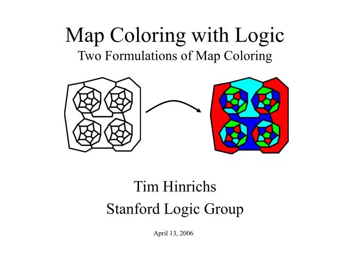
Map Coloring with LogicTwo Formulations of Map Coloring Tim Hinrichs Stanford Logic Group
Map Coloring Map Coloring with Logic
Map Coloring • Color the nodes of the graph so that • no two adjacent nodes are the same color Map Coloring with Logic
Map Coloring • Color the nodes of the graph so that • no two adjacent nodes are the same color Map Coloring with Logic
r3 r6 r4 r2 r5 r1 Student Formulation Premises: color(X,C) => region(X) color(X,C) => hue(C) adjacent(X1,X2) ^ color(X1,C) => -color(X2,C) region(X) => Y.color(X,Y) <ground atoms for adjacent, region, hue> Query: TUVXYZ | color(r1,T) ^ color(r2,U) ^ color(r3,V) ^ … • - This is not the formulation used in the CSP/LP literature. • - LP engines today do not understand this formulation. Map Coloring with Logic
r3 r6 r4 r2 r5 r1 Logic Programming Formulation • Axioms next(red,blue) next(red,green) next(red,yellow) next(blue,red) next(blue,green) … • Query R1 R2 R3 R4 R5 R6 | next(R1,R2) ^ next(R1,R3) ^ next(R1,R5) ^ next(R1,R6) ^ next(R2,R3) ^ next(R2,R4) ^ next(R2,R5) ^ next(R2,R6) ^ next(R3,R4) ^ next(R3,R6) ^ next(R5,R6) This is the typical formulation used in the literature. This form (deductive) is required by LP. Map Coloring with Logic
Map Coloring with Logic • Two formulations • The one students produce in CS157 every year • The one used in the literature [McCarthy82] • (1) is more natural (and non-deductive) (2) is more efficient (and deductive) • Question for the day: • How do we translate (1) into (2)? Map Coloring with Logic
Agenda • Consistency to Deduction: Reformulate non-deductive problem into deductive problem (a form of closing a theory) • Database Reformulation: turn output of (1) into the Logic Programming formulation. • Bilevel Reasoning: speeding up (1) Map Coloring with Logic
Running Example • Example: a very simple graph and two colors • 3 nodes, 2 edges • red and blue Problem: Solutions: Map Coloring with Logic
Constraint Satisfaction • Definition (Constraint Satisfaction Problem): Input: <V, DV, CV> V: set of variables v1,v2,… DV: domain for each variable -- dom(vi) CV: constraints on values of variables Output: Assignment of values to variables so that 1. val(vi) in dom(vi) 2. all the constraints are satisfied Map Coloring with Logic
Map Coloring as a CSP • Variables (V): nodes • Domains (DV): same for each variable for every i, dom(vi) = the set of colors • Constraints (CV): mathematically, a set of permissible tables, i.e. for every pair of variables x and y, a table for all the allowed values of x and y. Map Coloring with Logic
Example V: {R1, R2, R3} DV: dom(R1) = {r, b} dom(R2) = {r, b} dom(R3) = {r, b} r1 r2 r3 CV: Map Coloring with Logic
Example Solution V: {R1, R2, R3} DV: dom(R1) = {r, b} dom(R2) = {r, b} dom(R3) = {r, b} r1 r2 r3 CV: Map Coloring with Logic
All Solutions V: {R1, R2, R3} DV: dom(R1) = {r, b} dom(R2) = {r, b} dom(R3) = {r, b} r1 r2 r3 CV: Map Coloring with Logic
All Solutions as a DB Query • The set of all solutions can also be computed using the natural join operator. r1 r2 r3 = Map Coloring with Logic
Constraint Representations • Representing constraints as permissible tables can be expensive and cumbersome. • Often, constraints are more naturally and economically represented as logical sentences. Map Coloring with Logic
r1 r2 r3 Student Formulation Premises: color(X,C) => region(X) color(X,C) => hue(C) adjacent(X1,X2) ^ color(X1,C) => -color(X2,C) region(X) => Y.color(X,Y) adjacent(r1,r2) ^ adjacent(r2,r3) ^ hue(r) ^ hue(b) region(r1) ^ region(r2) ^ region(r3) Entailment Query: XYZ | color(r1,X) ^ color(r2,Y) ^ color(r3,Z) Models: Map Coloring with Logic
r1 r2 r3 Student Formulation Premises: color(X,C) => region(X) color(X,C) => hue(C) adjacent(X1,X2) ^ color(X1,C) => -color(X2,C) region(X) => Y.color(X,Y) adjacent(r1,r2) ^ adjacent(r2,r3) ^ hue(r) ^ hue(b) region(r1) ^ region(r2) ^ region(r3) Build a model: XYZ | color(r1,X) ^ color(r2,Y) ^ color(r3,Z) Models: Map Coloring with Logic
Logic Programming Formulation • Is different than the student formulation • [McCarthy82] borrowed from Pereira and Porto [1980] • McCarthy started with their formulation and showed various reformulations that improved efficiency. • Served as an exploration of Kowalski’s doctrine: Algorithm = Logic + Control • Originally used to illustrate issues in Constraint Satisfaction/Logic Programming Map Coloring with Logic
LP Formulation • Axioms next(r,b) next(b,r) • Entailment query R1 R2 R3 | next(R1,R2) ^ next(R2,R3) r1 r2 r3 Deductive Map Coloring with Logic
Problem Statement • Produce an algorithm that converts Axioms: color(X,C) => region(X) color(X,C) => hue(C) adjacent(X1,X2) ^ color(X1,C) => -color(X2,C) region(X) => Y.color(X,Y) … Build Model: XYZ |color(r1,X) ^ color(r2,Y) ^ color(r3,Z) into Axioms: next(red,blue) next(blue,red) Entailment Query: XYZ |next(X,Y) ^ next(Y,Z) Map Coloring with Logic
Herbrand Logic • Assume no function constants • The axioms include a • DCA over all ground terms • UNA over all ground terms • Assume these hold implicitly • Finite Herbrand Logic Map Coloring with Logic
An Observation: Student color(X,C) => region(X) color(X,C) => hue(C) adjacent(X,Y) ^ color(X,C) => -color(Y,C) • Write the last with V instead of => -adjacent(X,Y) V -color(X,C) V -color(Y,C) • Except for typing, these constraints are entirely negative • Entail what colorings are invalid. • Every other coloring is valid. Map Coloring with Logic
Student Colorings adjacent(X,Y) ^ color(X,C) => -color(Y,C) • Invalid answers (entailed) XYZ | -(color(r1,X) ^ color(r2,Y) ^ color(r3,Z)) • Remaining answers … Map Coloring with Logic
Idea • To reformulate from Student to LP, • Compute all invalid colorings (which are entailed). • Compute the complement of that set. = … Map Coloring with Logic
Implementation : the set of Student constraints Query: color(r1,X) ^ color(r2,Y) ^ color(r3,Z) • Reify the notion of an invalid coloring. (*) invalid(X,Y,Z) <=> -(color(r1,X) ^ color(r2,Y) ^ color(r3,Z)) • Ask for all the invalid colorings that are logically entailed. XYZ | ^ (*) |= invalid(X,Y,Z) Map Coloring with Logic
Implementation XYZ | invalid(X,Y,Z) • The following expression is logically entailed and represents the set of all invalid colorings: X=r1 v X=r2 v X=r3 v Y=r1 v Y=r2 v Y=r3 v Z=r1 v Z=r2 v Z=r3 v X=Y v Y=Z X Y Z Map Coloring with Logic
Implementation • To compute an expression that represents the complement of that set, it turns out that all we need to do is negate that expression. X≠r1 ^ X≠r2 ^ X≠r3 ^ Y≠r1 ^ Y≠r2 ^ Y≠r3 ^ Z≠r1 ^ Z≠r2 ^ Z≠r3 ^ X≠Y ^ Y≠Z • The above (with unique names axioms) entails all the valid colorings. X Y Z Map Coloring with Logic
Progress: Both are deductive • Student after reformulation: all deductive answers to XYZ | X≠r1 ^ X≠r2 ^ X≠r3 ^ Y≠r1 ^ Y≠r2 ^ Y≠r3 ^ Z≠r1 ^ Z≠r2 ^ Z≠r3 ^ X≠Z ^ Y≠Z UNA[r,b,r1,r2,r3] • LP formulation: all deductive answers to XYZ | next(X,Y) ^ next(Y,Z) next(r,b) next(b,r) X Y Z Map Coloring with Logic
Because Student* is now a query over a complete theory (≠), it can be viewed as a DB query. XYZ | X≠r1 ^ X≠r2 ^ X≠r3 ^ Y≠r1 ^ Y≠r2 ^ Y≠r3 ^ Z≠r1 ^ Z≠r2 ^ Z≠r3 ^ X≠Z ^ Y≠Z Student* as Database Query ≠ Map Coloring with Logic
Database Reformulation • Given one database query, find an equivalent query that is more efficient. • Includes performing transformations on the data itself, with a space limit. • Theorem [Chirkova]: There are infinitely many distinct transformations. • Theorem [Chirkova]: There is an algorithm that given the query constructs a finite space of queries that is guaranteed to include the optimal one. Map Coloring with Logic
X Y Z Back to Map Coloring • Given the query X≠r1 ^ X≠r2 ^ X≠r3 ^ Y≠r1 ^ … Z≠r3 ^ X≠Y ^ Y≠Z one of the transformations Chirkova’s work considers is view(X,Y) <= X≠r1 ^ X≠r2 ^ X≠r3 ^ Y≠r1 ^ Y≠r2 ^ Y≠r3 ^ X≠Y which can be used to rewrite the above query as view(X,Y) ^ view(Y,Z) Map Coloring with Logic
X Y Z Comparison • Student** XYZ | view(X,Y) ^ view(Y,Z) view(r,b) view(b,r) • Logic Programming XYZ | next(X,Y) ^ next(Y,Z) next(r,b) next(b,r) Map Coloring with Logic
Overview • Starting with the Student formulation, XYZ | color(r1,X) ^ color(r2,Y) ^ color(r3,Z) color(X,C) => region(X) color(X,C) => hue(C) adjacent(X1,X2) ^ color(X1,C) => -color(X2,C) use logical entailment to find an expression for all the invalid colorings and negate it. XYZ | X≠r1 ^ X≠r2 ^ X≠r3 ^ … ^ X≠Y ^ Y≠Z • Then apply Chirkova’s work to produce the LP formulation, or one that is at least as good as LP. XYZ | view(X,Y) ^ view(Y,Z) Map Coloring with Logic
Another Example • N-Queens: place N queens on an NxN chessboard s.t. • No queen can be attacked by another queen. That is • No two queens share the same row • No two queens share the same column • No two queens share the same diagonal Map Coloring with Logic
8 Queens Solution Map Coloring with Logic
N-Queens Constraints • All queens in different rows X≠Y ^ row(X,R) => -row(Y,R) • All queens in different columns X≠Y ^ col(X,C) => -col(Y,C) • All queens in different diagonals X≠Y ^ diag(X,D1,D2) => -diag(Y,D1,D2) Map Coloring with Logic
N-Queens Diagonals • Row, Col is enough to compute the two diagonals diag(X,pos,D) <= row(X,R) ^ col(X,C) ^ sub(C, R, D) diag(X,neg,D) <= row(X,R) ^ col(X,C) ^ add(C, R, D) • Diagonals represented by their slope and y-intercepts 4 3 2 1 0 Map Coloring with Logic
4 Queens Query • Satisfiability Query: (X1 Y1 X2 Y2 X3 Y3 X4 Y4) | row(q1,X1) ^ col(q1,Y1) ^ row(q2,X2) ^ col(q2,Y2) ^ row(q3,X3) ^ col(q3,Y3) ^ row(q4,X4) ^ col(q4,Y4) Map Coloring with Logic
Efficiency in N-Queens • The expression that represents all invalid positions can become quite large and might take a long time to compute because of the add and sub facts. • About 150 conjuncts • Idea: produce an expression in terms of add and sub, as well as =. Map Coloring with Logic
Bilevel Reasoning • Separate constraints from data. • X≠Y ^ row(X,R) => -row(Y,R) • X≠Y ^ col(X,C) => -col(Y,C) • X≠Y ^ diag(X,D1,D2) => -diag(Y,D1,D2) • diag(X,pos,D) <= row(X,R) ^ col(X,C) ^ sub(C, R, D) • diag(X,neg,D) <= row(X,R) ^ col(X,C) ^ add(C, R, D) • add(1,1,2) • add(1,1,3) • ... • add(4,4,8) • sub(1,1,0) • sub(1,2,-1) • ... • sub(4,4,0) Map Coloring with Logic
Bilevel Reasoning • Separate constraints from data. • X≠Y ^ row(X,R) => -row(Y,R) • X≠Y ^ col(X,C) => -col(Y,C) • X≠Y ^ diag(X,D1,D2) => -diag(Y,D1,D2) • diag(X,pos,D) <= row(X,R) ^ col(X,C) ^ sub(C, R, D) • diag(X,neg,D) <= row(X,R) ^ col(X,C) ^ add(C, R, D) • add(1,1,2) • add(1,1,3) • ... • add(4,4,8) • sub(1,1,0) • sub(1,2,-1) • ... • sub(4,4,0) Map Coloring with Logic
Bilevel Reasoning • Separate constraints from data. • X≠Y ^ row(X,R) => -row(Y,R) • X≠Y ^ col(X,C) => -col(Y,C) • X≠Y ^ diag(X,D1,D2) => -diag(Y,D1,D2) • diag(X,pos,D) <= row(X,R) ^ col(X,C) ^ sub(C, R, D) • diag(X,neg,D) <= row(X,R) ^ col(X,C) ^ add(C, R, D) • add(1,1,2) • add(1,1,3) • ... • add(4,4,8) • sub(1,1,0) • sub(1,2,-1) • ... • sub(4,4,0) Map Coloring with Logic
Implementation ’: the set of n-queens constraints w/o add/sub Query: row(q1,X1) ^ col(q2,Y1) ^ row(q3,X2) ^ ... • Reify the notion of an invalid coloring. (*) invalid(X1,Y1,X2,Y2,X3,Y3,X4,Y4) <=> -(row(q1,X1) ^ col(q2,Y1) ^ row(q3,X2) ^ ...) • Ask for all the invalid colorings where add/sub can be assumed, i.e. use residues (a form of abduction). XYZ | ’ ^ (*) |= invalid(X,Y,Z) Map Coloring with Logic
4-Queens Partial Reformulation goal(X1,Y1,X2,Y2,X3,Y3,X4,Y4) <= X1 ≠ X2 Y1 ≠ Y2 (-sub(Y2,X2,Z) v -sub(Y1,X1,Z)) (-add(Y2,X2,Z)) v -add(Y1,X1,Z)) X1 ≠ X3 Y1 ≠ Y3 X2 ≠ X3 Y2 ≠ Y3 (-sub(Y3,X3,Z) v -sub(Y1,X1,Z)) (-sub(Y3,X3,Z) v -sub(Y2,X2,Z)) (-add(Y3,X3,Z) v -add(Y1,X1,Z)) (-add(Y3,X3,Z) v -add(Y2,X2,Z)) ... Map Coloring with Logic
Consistency to Deduction • Computing the sentences that are consistent with the premises and making them deductive consequences. • Definition (query consistency to deduction): qC2D[, (xbar)] = {tbar | (tbar) is satisfiable} • In map coloring, = the set of map coloring axioms (xbar) = color(r1,X) ^ color(r2,Y) ^ color(r3,Z) qC2D = {<r,b,r>, <b,r,b>} Map Coloring with Logic
Descriptions • Definition (Description): e(xbar) is a description for the set of n-tuples S, where |xbar| = n if and only if |= e(tbar) if tbar S |= -e(tbar) if tbar S • Example: X=Y V Y=Z describes {rrr,rrb,brr,bbr,rbb,bbb} in FHL |=H r=r V r=r |=H r=r V r=b |=H b=r V r=r |=H b=b V b=r |=H r=b V b=b |=H b=b V b=b and |=H -(r=b V b=r) |=H -(b=r V r=b) Map Coloring with Logic
Algorithm • Input : a finite set of FHL sentences (xbar): a query in the vocabulary of Delta • Using algorithm Alg, compute an expression e(xbar) in terms of equality such that for any model M in R, |=M e(tbar) if and only if |= -(tbar) • Output -e(xbar) Map Coloring with Logic
Theorems • Theorem (Soundness and Completeness): Let Alg(, (xbar)) = -e(xbar). |=M -e(tbar) if and only if (tbar) qC2D[, (xbar)] Proof: Nontrivial • Theorem (Decidability): qC2D[, (xbar)] for FHL is decidable. Proof: Walk over Herbrand models and if |=M , collect all tbar s.t. |=M (tbar) Map Coloring with Logic
Relationship to CWA • CWA[] includes -p(tbar) whenever |# p(tbar) • CWA[] is inconsistent whenever • Delta entails some disjunction d1 v … v dn and • Delta entails none of the di. • Adding the map coloring answers to the Student formulation is inconsistent. Map Coloring with Logic


![[PDF] COLORING BOOK OF MAGIC: Coloring book of magic. Adult coloring book with p](https://cdn7.slideserve.com/12431398/slide1-dt.jpg)