Download
1 / 37
370 likes | 966 Views
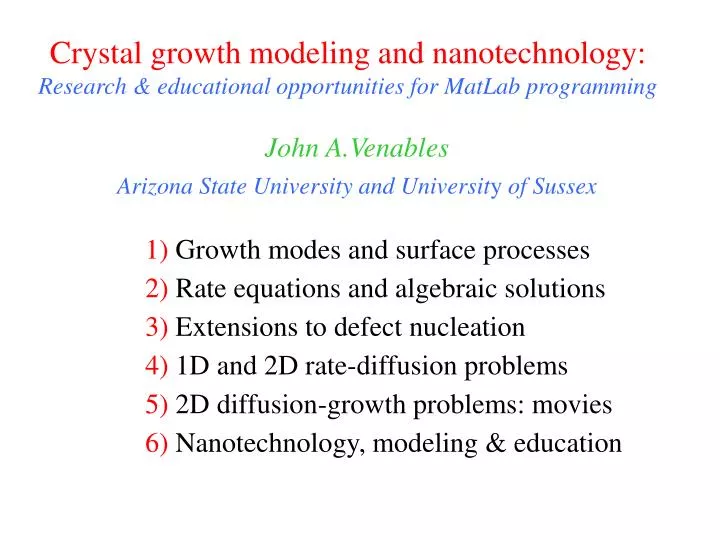
Crystal growth modeling and nanotechnology: Research & educational opportunities for MatLab programming. John A.Venables Arizona State University and Universit y of Sussex. 1) Growth modes and surface processes 2) Rate equations and algebraic solutions 3) Extensions to defect nucleation

E N D
Crystal growth modeling and nanotechnology:Research & educational opportunities for MatLab programming John A.Venables Arizona State University and University of Sussex 1) Growth modes and surface processes 2) Rate equations and algebraic solutions 3) Extensions to defect nucleation 4) 1D and 2D rate-diffusion problems 5) 2D diffusion-growth problems: movies 6) Nanotechnology, modeling & education
Explanation for NAN 546: April 09 This talk was given at several departmental seminars in the period 2003-05. These seminars typically require about 40-50 minutes and this one has 36 slides (#1, 3-37 here), with none in reserve this time. The audience is usually a Materials Department, with the level aimed at the Graduate Students Slide #3 is an Agenda slide to guide one through the talk. The hyperlinks on slide #1 connect to Custom Shows, available under the Slide Show dropdown menu. This particular talk has a tutorial character, which explains why we have been able to use it for sessions on growth modes, diffusion mechanisms, rate equations, stress effects, visualization, etc This material is copyright of John A. Venables. Author and Journal references are typically given in green, and I do not talk about material that has not been published in some form.
Crystal growth modeling & nanotechnology:Research & educational opportunities for MatLab programming John A.Venables Arizona State University and LCN-UCL • Growth modes and surface processes • Rate equations and algebraic solutions • Extensions to defect nucleation • 1D and 2D rate-diffusion problems • 2D diffusion-growth problems: movies • Nanotechnology, modeling & education
Growth modes IslandLayer + Island Layer Volmer-Weber Stranski-Krastanov Frank-VdM
Atomic-level processes Variables: R (or F), T, time sequences (t) Parameters: Ea, Ed, Eb, mobility, defects…
Early TEM pictures: Au/NaCl(001) Donohoe and Robins (1972) JCG
Alternative approaches to modeling Rate and diffusion equations Kinetic Monte Carlo simulations Level-set and related methods plus 4) Correlation with ab-initio calculations Issues:Length and time scales, multi-scale; Parameter sets, lumped parameters; Ratsch and Venables, JVST A S96-109 (2003)
Rate Equations(experimental variables T, F or R, t) dn1/dt = F(or R) –n1/t®n1(t), single adatoms .... dnj/dt = Uj-1 - Uj = 0 ®nj(t), via local equilibrium .... dnx/dt = ®å dnj/dt = Ui - ...®nx(t), (j > i +1) stable cluster density Ui = siDn1ni , with si , sx as capture numbers t–1 = siD(i+1)ni+ sxDnxnucleation, growth
Competitive capture dn1/dt = R (or F) – n1/t; t-1 = ta-1 + tn-1 + tc-1… Venables PRB 36 4153-62 (1987)
Differential equations versus Algebra Using cluster shape, assumed or measured, express nx(Z) ®h(Z). f1(Rpexp(E/kT)) t(Z) ®k(Z). f2(Rpexp(E/kT)); where p and E are functions of i,critical nucleus size similarly for mean size ax(Z) and condensation coefficient b(Z), not much used. Choice of 1) integrating differential equations, or 2) evaluating near the maximum of nx(Z). Steady state conditions (dnx/dt, etc = 0) converts a set of ODE’s into a (nonlinear) algebraic solution.
Nucleation density predictions • Matlab Programs (R, T-1 and cluster size, j) • Input Energies • Simultaneous output: Densities and critical cluster size, i. McDaniels et al. PRL 87 (2001) 176105, data, and work in progress on rate equation and 2D modeling
Nucleation on point and line defects (a) Point defects (vacancies) (b) Line defects (steps)
Extension to Defect Nucleation (parameters nt, Et) dn1/dt = R –n1/t®n1(t), single terrace adatoms dn1t/dt = s1tDn1nte - n1tndexp(-(Et+Ed)/kT) ®n1t(t) ....empty traps trapped adatoms dnj/dt = Uj-1 - Uj = 0 ®nj(t), via local equilibrium dnj’t/dt®nj’t(t), not necessarily samei, i’ .... dnx/dt = ®å dnj/dt = Ui - ...®nx(t), (j > i +1) terrace cluster density dnxt/dt = ®å dnj’t/dt = Ui’t - ...®nxt(t), (j’ > i’ +1) trapped cluster density
Point defects and Nanofabrication? For Fe/CaF2(111):Heim et al. 1996, JAP; Venables 1999
A particular case:Pd/MgO (001) Defect nucleation, i = 3 at high T Haas et al. 2000 PRB; Venables and Harding 2000 JCG
More complex situations: 1D and 2D rate-diffusion equations Examples so far: dn1/dt, dnx/dt®n1(t), nx(Z), etc., all spatial averages Next, linear or radial 1D problems: capture numbers, step capture, deposition past a mask, quantum wires
Capture numbers:1D radial rate-diffusion equations dn1(r,t)/dt = G(r,t) –n1(r,t)/t(r,t) +Ñ.[D(r)Ñn1(r,t)] G(r,t),generation rate ®n1(r, t), adatom profile dnx(r,t)/dt = å dnj(r,t)/dt = Ui(r,t) – ...®nx(r, t) ®nx(r, t) stable cluster density profile Deals with deposition (G~F) and annealing (G~0), plus also potential energy landscapes, V(r), via Nernst- Einstein equation (t-dependence implicit), j(r) = –D(r)Ñn1(r) – [n1(r)D*(r)]bÑV(r) radial current ® s capture number
Diffusion and attachment limits Diffusion solution, at r = rk+ r0 sD = 2pXk0.(K1(Xk0)/ K0(Xk0)), with Xk0 = (rk+ r0)/(D1t)1/2 Attachment (barrier) solution: sB = 2p(rk+ r0)exp(-bEB) = B(rk+ r0) or BV(rk+ r0) They combine inversely as sk -1 = sB-1 + sD-1 a) B=2pexp(-bEB) b) BV=2pexp(-bV0) Venables and Brune PRB 66 (2002) 195404
Delayed onset of nucleation Reduced capture numbers: longer transient regime (nx) Venables and Brune 2002
Repulsive adsorbate interactions: Cu/Cu(111) Annealing, low T (16.5K),Cu/Cu(111) Rate equations, full lines as f (rd); KMC, squares with error bars. Cu/Cu(111): STM, 0.0014 ML, preferred spacing Knorr et al. PRB 65 (2002) 115420; Venables & Brune (2002) PRB
Interpolation scheme for annealing: i = 1 Full lines: Attachment limit Dashed lines: Diffusion limit Previous slides: Interpolation dn1/d(D1t) = -2s1n12 -sxn1nx, dnx/d(D1t) = s1n12, with sk = sinit ft + skd(1-ft), sinit = sBft; ft = K0(Xd)/K0(Xk0); Xd = (rk+r0+rd)/(D1t)1/2 with time-dependent rd = (0.5D1t)1/2BV/2p.
Extrapolation to higher temperatures REs:integrate to 2 or 20 min. anneal with givenV0. KMC: hexagonal lattice simulations (1000 x 1155) sites with EB = V0. Compare KMC-STM: 10 < V0 < 14 meV;Venables & Brune 2002
Extension to Ge/Si(001)stress-limited capture numbers • Low dimer formation energy (Ef2 ~ 0.35 eV) gives large i, even though condensation is complete • Stress grows with island size, sx decreases • Lengthened transient regime results, > 1 ML, source of very mobile ad-dimers (Ed2 ~ 1 eV) for rapid growth eventually of dislocated islands • Interdiffusion, and diffusion away from high stress regions around islands, reduces stress at higher T and lower F (e.g. at 600, not 450 oC for F ~1-3 ML/min.) Chaparro et al.JAP 2000, Venables et al.Roy. Soc. A361 (2003) 311
Conclusions: t-dependent capture numbers 1) Explicit t-dependence involves the transient regime and a finite number of adatoms. Barriers or repulsive potential fields reduce capture numbers, lengthen transients and involve more adatoms. 2)Barrier capture numbers and diffusion capture numbers add inversely. An interpolation scheme is needed to describe t-dependence in the transient. 3)Large critical nucleus size lengthens transient. Annealing a low T deposit with potential fields is a very sensitive test of t-dependent capture numbers, as small capture numbers result in little annealing.
And finally, Area 2D (x,y,t or r,f,t) problems: Shapes, edge diffusion, instabilities, lithography, quantum dots, anisotropic stress effects, etc. Geometries to consider are square or rectangular, using an (x,y) mesh: e.g. (2x1) and (1x2) Si(001); hexagonal, which can be approximated by a 1D cylindrical (r) domain; triangular lattice, applicable to reconstructed f.c.c. metal and semiconductor (111) surfaces. Expts: STM of Co/Si(111); and Ag/Ag layers/Pt(111) (Bennett et al.) (Brune et al.)
Questions for 1D and 2D modelling 1) How far can one realistically go without becoming over-dependent on too many unknown parameters?? 2)How many types of different experiments can one actually perform? 3)Large-scale (commercial) packages can solve PDEs.But, is the science unique, or do multiple inputs give the same results? • Importance of lumped parameters
FFT Method for time-dependent x-y Diffusion Fields The general solution to on a rectangular grid (X,Y) (kx, ky points) is C = Field = ifft2(fft2(Field).*Pmat) where the propagator Pmat for time Dt is: unitmat.* exp(-2Dt(DX(1-cos(2p(X-1)/kx))/a2 + DY(1-cos(2p(Y-1)/ky)))/b2)
Program Structure (MatLabâ 6.5) • Initialize, set up Field and Island Masks • Calculate Propagator, Pmat, for Dt • Loop over time steps: ktimes = [1:900] • Update Field, calculate fluxes and reset boundary conditions on Island and Field • Plot Field data at plottime = [1 2.. 10.. 900] • Save calculated capture number data & other calculations for subsequent plotting
Annealing: rectangular islands height = 5 time = 90 Dt = 0.1 64*64 grid (5*11) grows to (19*33) Dx = 5 Dy = 10 Venables & Yang 2004
1D and 2D results and conclusions • Attachment-limited solutions EB, V(r) for STM Cu/Cu(111)Brune (EPFL), Phys. Rev. B 2002; AFM Ge/Si(001) Drucker (ASU), in progress • Anisotropic attachment and growth: AFM/STM/ LEEM/HREM (Co,Pd) silicide nanowiresBennett • Anisotropic 2D nucleation and growth: AFM/ LEEM/HREM Ag/Si nanowiresLi & Zuo (UIUC) Conclusion: It is worth exploring a few models with a few defined parameters in 1 and 2 spatial dimensions when a strong connection to experiment is available.
Nanotechnology, modeling & education • Interest in crystal growth, atomistic models and experiments in collaboration • Interest in graduate education: web-based, web-enhanced courses, book • See http://venables.asu.edu/ for details • Opportunities for undergraduate (REU), and graduate projects as part of M.S, Ph.D
Pattern formation: magnetic wires Sugawara et al. (1997) APL, JAP Fe/SiO/NaCl(110): Anisotropic magnet, MOKE, Holography
Optical properties of InGaAs/GaAs Modeling, TEM, EELS, PL: Shumway, Zunger, Catalano, Crozier et al. PRB ‘01
Size and position uniformityin stacked PbSe/PbEuTe QDSL’s AFM, almost hexagonal ordering, see FFT insert: Raab, Lechner, Springholz, APL ’02 & refs quoted
Nanotechnology: alternative routes Optical superlattice: CdSe Magnetic superlattice Ag/Co Murray et al., 1995++, Science Sun & Murray, 1999+, JAP
Nanotechnology, modeling & education • Interest in crystal growth, atomistic models and experiments in collaboration • Interest in graduate education: web-based, web-enhanced courses, book • See http://venables.asu.edu/ for details • Opportunities for undergraduate (REU), and graduate projects as part of M.S, Ph.D