Download
1 / 21
230 likes | 385 Views
Time Series Building. 1. Model Identification. Simple time series plot : preliminary assessment tool for stationarity Non stationarity : consider time series plot of first ( d th ) differences Unit root test of Dickey & Fuller : check for the need of differencing

E N D
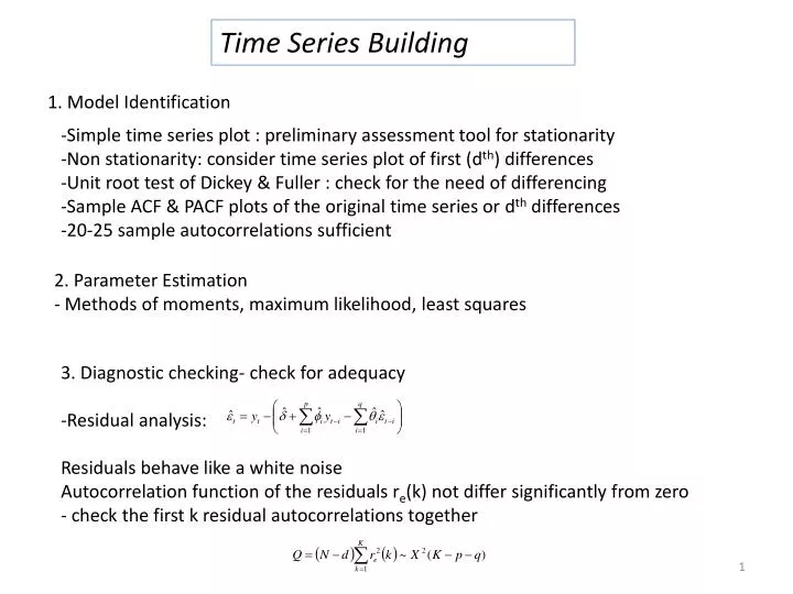
Time Series Building 1. Model Identification • Simple time series plot : preliminary assessment tool for stationarity • Non stationarity: consider time series plot of first (dth) differences • Unit root test of Dickey & Fuller : check for the need of differencing • Sample ACF & PACF plots of the original time series or dth differences • 20-25 sample autocorrelations sufficient 2. Parameter Estimation - Methods of moments, maximum likelihood, least squares • 3. Diagnostic checking- check for adequacy • Residual analysis: • Residuals behave like a white noise • Autocorrelation function of the residuals re(k) not differ significantly from zero- check the first k residual autocorrelations together
Example May exist some autocorrelation between the number of applications in the current week & the number of loan applications in the previous weeks
Weekly data: • Short runs • Autocorrelation • A slight drop in the mean for the 2nd year (53-104 weeks) : • Safe to assume stationarity • Sample ACF plot: • Cuts off after lag 2 (or 3) • MA(2) or MA(3) model • - Exponential decay pattern • AR(p) model • Sample PACF plot: • Cuts off after lag 2 • Use AR(2) model
- Parameter estimates: Significant - Box-Pierce test: no autocorrelation -sample ACF & PACF: confirm also
Acceptable fit Fitted values: smooth out the highs and lows in the data
Example • Signs of non-stationarity: • changing mean & variance • Sample ACF: slow decreasing • Sample PACF: significant value at lag 1, close to 1 Significant sample PACF value at lag 1: AR(1) model
Residuals plot: changing variance - Violates the constant variance assumption
- AR(1) model coefficient: Significant - Box-Pierce test: no autocorrelation -sample ACF & PACF: confirm also
Plot of the first difference: -level of the first difference remains the same Sample ACF & PACF plots: first difference white noise RANDOM WALK MODEL, ARIMA(0,1,0)
Decide between the 2 models AR(1) & ARIMA(0,1,0) • Use specific criteria • Use subjective matter /process knowledge Do we expect a financial index as the Dow Jones Index to be around a fixed mean, as implied by AR(1)? ARIMA(0,1,0) takes into account the inherent non stationarity of the process However A random walk model means the price changes are random and cannot be predicted Not reliable and effective forecasting model Random walks models for financial data
Forecast ARIMA process How to obtain Best forecast The mean square error for which the expected value of the squared forecast errors is minimized Best forecast in the mean square sense Forecast error
Mean & variance Variance of the forecast errors: bigger with increasing forecast lead times Prediction Intervals 100(1-a) percent prediction interval
2problems • Infinite many terms in the past, in practice have finite number of data • Need to know the magnitude of random shocks in the past • Estimate past random shocks through one-step forecasts ARIMA model
forecast ARIMA(1,1,1) process 1. Infinite MA representation of the model forecast weights Random shocks
Seasonality in a time series is a regular pattern of changes that repeats over S time periods, where S defines the number of time periods until the pattern repeats again.
SEASONAL PROCESS St deterministic with periodicity s Nt stochastic, modeled ARMA wt seasonally stationary process Model Nt with ARMA becomes stationary Assume after seasonal differencing Seasonal ARMA model
Example • Monthly seasonality, s=12: • ACF values at lags 12, 24,36 are significant & slowly decreasing • PACF values: lag 12 significant value close to 1 • Non-stationarity: slowly decreasing ACF • Remedy of non-stationarity: take first differences & seasonal differencing • Eliminates seasonality • stationary Sample ACF: significant value at lag 1 Sample PACF : exponentially decaying values at the first 8 lags Use non seasonal MA(1) model Remaining seasonality: Sample ACF: significant value at lag 12 Sample PACF : lags 12, 24,36 alternate in sign Use seasonal MA(1) model
ARIMA(0,1,1)x(0,1,1)12 Coefficient estimates: MA(1) & seasonal MA(1) significant Sample ACF & PACF plots: still some significant values Box-Pierce statistic: most of the autocorrelation is out