Download
1 / 18
180 likes | 297 Views
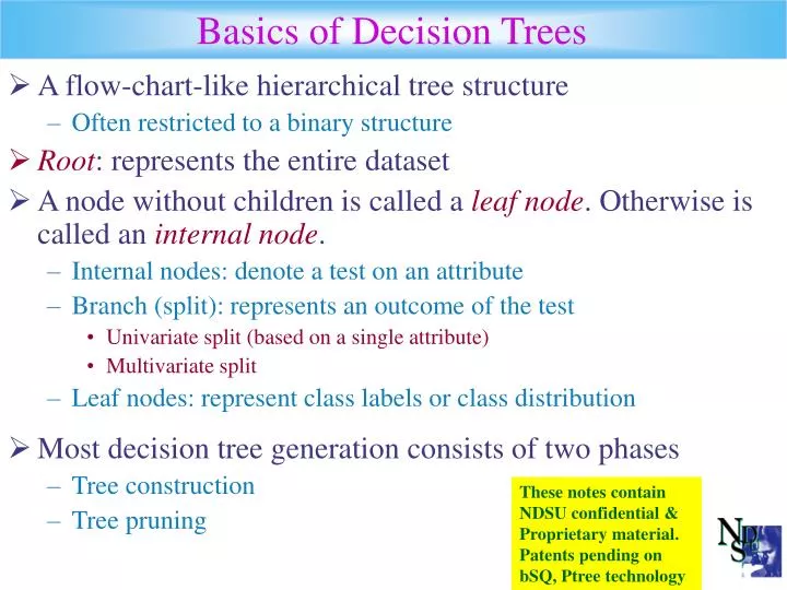
Basics of Decision Trees . A flow-chart-like hierarchical tree structure Often restricted to a binary structure Root : represents the entire dataset A node without children is called a leaf node . Otherwise is called an internal node . Internal nodes: denote a test on an attribute

E N D
Basics of Decision Trees • A flow-chart-like hierarchical tree structure • Often restricted to a binary structure • Root: represents the entire dataset • A node without children is called a leaf node. Otherwise is called an internal node. • Internal nodes: denote a test on an attribute • Branch (split): represents an outcome of the test • Univariate split (based on a single attribute) • Multivariate split • Leaf nodes: represent class labels or class distribution • Most decision tree generation consists of two phases • Tree construction • Tree pruning These notes contain NDSU confidential & Proprietary material. Patents pending on bSQ, Ptree technology
Example (training dataset) Record ID Salary Age Employment Group 1 30K 30 Self C 2 40K 35 Industry C 3 70K 50 Academia C 4 60K 45 Self B 5 70K 30 Academia B 6 60K 35 Industry A 7 60K 35 Self A 8 70K 30 Self A 9 40K 45 Industry C • Three predictor attributes: salary, age, employment • Class label attribute: group
Example (univariate split) Salary <= 50K > 50K Group C Age <= 40 > 40 Group C Employment Academia, Industry Self Group B Group A • Each internal node of a decision tree is labeled with a predictor attribute, called the splitting attribute • each leaf node is labeled with a class label. • Each edge originating from an internal node is labeled with a splitting predicate that involves only the node’s splitting attribute. • The combined information about splitting attributes and splitting predicates at a node is called the split criterion
Building Decision Trees • Basic algorithm (a greedy algorithm) • Tree is constructed in a top-down recursive divide-and-conquer manner • At start, all the training examples are at the root • Attributes are categorical (if continuous-valued, they are discritized in advance) • Examples are partitioned recursively based on selected attributes • Test attributes are selected on the basis of a heuristic or statistical measure (e.g., information gain)
Tree-Building Algorithm • We can build the whole tree by calling: BuildTree(dataset TrainingData, split-selection-method CL) Input: dataset S, split-selection-method CL Output: decision tree for S Top-Down Decision Tree Induction Schema (Binary Splits): BuildTree(dataset S, split-selection-method CL) (1) If (all points in S are in the same class) then return; (2) Using CL to evaluate splits for each attribute (3) Use best split found to partition S into S1 and S2; (4) BuildTree(S1, CL) (5) BuildTree(S2, CL)
Split Selection • Information gain / Gain ratio (ID3/C4.5) • All attributes are assumed to be categorical • Can be modified for continuous-valued attributes • Gini index (IBM IntelligentMiner) • All attributes are assumed continuous-valued • Assume there exist several possible split values for each attribute • May need other tools, such as clustering, to get the possible split values • Can be modified for categorical attributes
Information Gain (ID3) • T – Training set; S – any set of cases • freq(Ci, S) – the number of cases that belong to class Ci • |S| -- the number of cases in set S • Information of set S is defined: • consider a similar measurement after T has been partitioned in accordance with the n outcomes of a test X. The expected information requirement can be found as the weighted sum over the subsets, as • The quantity measures the information that is gained by partitioning T in accordance with the test X. The gain criterion, then, selects a test to maximize this information gain. gain(X) = info(T) – infoX(T)
Gain Ratio (C4.5) • Gain criterion has a serious deficiency – it has a strong bias in favor of tests with many outcomes. • We have This represents the potential information generated by dividing T into n subsets, whereas the information gain measures the information relevant to classification that arises from the same division. • Then, expresses the proportion of information generated by the split that is useful, i.e., that appears helpful for classification. Gain ratio(X) = gain(X)/split info(X)
Gini Index (IBM IntelligentMiner) • If a data set T contains examples from n classes, gini index, gini(T) is defined as where pj is the relative frequency of class j in T. • If a data set T is split into two subsets T1 and T2 with sizes N1 and N2 respectively, the gini index of the split data contains examples from n classes, the gini index gini(T) is defined as • The attribute provides the smallest ginisplit(T) is chosen to split the node (need to enumerate all possible splitting points for each attribute).
Pruning Decision Trees • Why prune? • Overfitting • Too many branches, some may reflect anomalies due to noise or outliers • Result is in poor accuracy for unseen samples • Two approaches to prune • Prepruning: Halt tree construction early—do not split a node if this would result in the goodness measure falling below a threshold • Difficult to choose an appropriate threshold • Postpruning: Remove branches from a “fully grown” tree—get a sequence of progressively pruned trees • Use set of data different from training data to decide “best pruned tree” • Well-known Pruning Methods: • Reduced Error Pruning Pessimistic Error Pruning • Minimum Error Pruning Critical Value Pruning • Cost-Complexity Pruning Error-Based Pruning
Extracting Rules from Decision Trees • Represent the knowledge in the form of IF-THEN rules • One rule is created for each path from the root to a leaf • Each attribute-value pair along a path forms a conjunction • The leaf node holds the class prediction • Rules are easier for humans to understand • Example • IF salary=“>50k” AND age=“>40” THEN group=“C”
Why Decision Tree Induction • Compared to a neural network or a Bayesian classifier, a decision tree is easily interpreted/comprehended by humans • While training neural networks can take large amounts of time and thousands of iterations, inducing decision trees is efficient and is thus suitable for large training sets • Decision tree generation algorithms do not require additional information besides that already contained in the training data • Decision trees display good classification accuracy compared to other techniques • Decision tree induction can use SQL queries for accessing databases
Tree Quality Measures • Accuracy • Complexity • Tree size • Number of leaf nodes • Computational speed • Scalability: Classifying data sets with millions of examples and hundreds of attributes with reasonable speed
Some Published Methods (can Ptrees improve speed/accuracy of these?) • SLIQ (EDBT’96 — Mehta et al.) • builds an index for each attribute and only class list and the current attribute list reside in memory • SPRINT (VLDB’96 — J. Shafer et al.) • constructs an attribute list data structure • PUBLIC (VLDB’98 — Rastogi & Shim) • integrates tree splitting and tree pruning: stop growing the tree earlier • RainForest (VLDB’98 — Gehrke, Ramakrishnan & Ganti) • separates the scalability aspects from the criteria that determine the quality of the tree • builds an AVC-list (attribute, value, class label) • BOAT • CLOUDS
Other Issues • Allow for continuous-valued attributes • Dynamically define new discrete-valued attributes that partition the continuous attribute value into a discrete set of intervals • Handle missing attribute values • Assign the most common value of the attribute • Assign probability to each of the possible values • Attribute (feature) construction • Create new attributes based on existing ones that are sparsely represented • This reduces fragmentation, repetition, and replication • Incremental tree induction • Integration of data warehousing techniques • Different data access methods • Bias in split selection
Decision Tree Induction Using P-trees • Basic Ideas • Calculate information gain, gain ratio or gini index by using the count information recorded in P-trees. • P-tree generation replaces sub-sample set creation. • Use P-tree to determine if all the samples are in the same class. • Without additional database scan
Using P-trees to CalculateInformation Gain/Gain Ratio • C – class label attribute • Ps – P-tree of set S • Freq(Cj, S) = rc{Ps ^ Pc(Vcj)} • |S| = rc{Ps} • |Ti| = rc{PT^P(VXi)} • |T| = rc{PT} • So every formula of Information Gain and Gain Ratio can be calculated directly using P-trees.
P-Classifier versus ID3 Classification cost with respect to the dataset size