Swiss Federal Institute of Aquatic Science and Technology Kastanienbaum - Switzerland

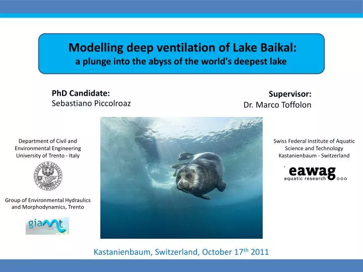
1. Modelling deep ventilation of Lake Baikal: a plunge into the abyss of the world's deepest lake Department of Civil and Environmental Engineering University of Trento - Italy Swiss Federal Institute of Aquatic Science and Technology Kastanienbaum - Switzerland Group of Environmental Hydraulics and Morphodynamics, Trento Kastanienbaum, Switzerland, October 17th 2011

2. Lake Baikal - introduction Lake Baikal - Siberia (Озеро Байкал - Сибирь) The lake of records The oldest, deepest and most voluminous lake in the world

3. Lake Baikal - introduction Lake Baikal in numbers Lake Baikal formed in an ancient rift valley  tectonic origin Divided into 3 sub-basins: South Basin Central Basin North Basin Main characteristics: Volume: 23 600 km3 Surface area: 31 700 km2 Length: 636 km Max. width: 79 km Max .depth: 1 642 m Ave. Depth: 744 m Shore Length:  2 100 km Surf. Elevation: 455.5 m Age: 25 million years Inflow rivers:  300 Outflow rivers: 1 (Angara River) World Heritage Site in 1996 1461 m

4. Lake Baikal - introduction Some curiosities The largest freshwater basin in the world: Freezes annually: Jan - May in the South Basin Dec - June in the North Basin 20% of the world’s total unfrozen fresh water reserve Surface area: 31 700 km2 Great Lakes are almost 8 times more extended than Lake Baikal but taken all together, have the same volume of water! Surface area: 244 160 km2

5. Lake Baikal - introduction The Pearl of Siberia 1/2 Singular, sometimes extreme, environmental conditions: • enormous depth • several months of ice cover • high oxygen concentration • low nutrient concentration gave rise to a unique ecosystem:  more than 1000 endemic species (diatoms, sponges, salmonid fish and the Baikal freshwater seal) An amphipod regards a diver from a sponge forest in Lake Baikal. It has been estimated that the biomass of crustaceans in the lake exceeds 1,800,000 tons Baikal oilfish (Golomyanka): a translucent abyssal fish famous for decomposing almost instantly to fat and bones when exposed to the sun Baikal seal or Nerpa (Pusa sibirica): the only exclusively freshwater pinniped species

6. Lake Baikal - introduction The bathymetry An impressive bathymetry: average depth at 744 m flat bottom steep sides

7. Deep ventilation Temperature [°C] 2 1 3 4 0 Tρmax Temperature profile 500 Reference parcel Depth [m] 1000 1500 Deep ventilation The physical mechanism • Phenomenon triggered by thermobaric instability (Weiss et al., 1991): • density depends on T and P (equation of state: Chen and Millero, 1976) • T of maximum density decreases with the depth (P=Patm Tρmax ≈ 4°C) Strong external forcing Weak external forcing ρparcel< ρlocal ρparcel = ρlocal ρparcel > ρlocal Compensation depth - hc

8. Deep ventilation A simplified sketch • The main effects: • deep water renewal; • a permanent, even if weak, stratified temperature profile. • high oxygen concentration up to the bottom; deep ventilation at the shore wind sinking volume of water Presence of aquatic life down to huge depths!

9. Deep ventilation The state of the art • Observations and data analysis: • Weiss et al., 1991; Killworth et al., 1996; Peeters et al., 1997, 2000; Wüest et al., 2005; Schmid et al., 2008 • Downwelling periods (May – June and December – January) • Downwelling temperature (3 ÷ 3.3 °C) • Downwelling volumes estimations (10 ÷ 100 per year) • Numerical simulations: • Akitomo, 1995; Walker and Watts, 1995; Tsvetova, 1999; Botte and Kay, 2002; Lawrence et al., 2002 • 2D or 3D numerical models • Simplified geometries or partial domains • Main aim: understand the phenomenon (triggering factors/conditions) Walker and Watts, 1995

10. A simplified 1D numerical model A simplified 1D model The aims • simple way to represent the phenomenon (at the basin scale) • just a few input data required (according to the available measurements) • suitable to predict long-term dynamics (i.e. climate change scenarios) The model in three parts • simplified downwelling mechanism (wind energy input vs energy required to reach hc) • lagrangian vertical stabilization algorithm (looking for unstable regions) • vertical diffusion equation solver with source terms (for temperature, oxygen and other solutes)

11. A simplified 1D numerical model The downwelling mechanism Hypsometric curve Temperature [°C] Constant-volume discretization scheme • Procedural steps: • assign Vd and ew • compute Td • calculate hc • compute the energy required to move Vd • move the Vd until zd • Two cases: • Shallow downwelling • Deep downwelling 3 3.5 Td 4 0 1 200 hc Vi-1 Vi Depth [m] Depth [m] Vi+1 Tρmax 1500 dT/dz|ad Vi = 5 km3 1272 sub-volumes Volume [km3]

12. A simplified 1D numerical model The lagrangian vertical stabilization algorithm The profile is unstable:  the sinking Vd is heavier (lighter) than the surrounding water Temperature [°C] 3 3.5 0 200 hc We need to stabilize the temperature profile mixing factor included to take into account the exchanges occurring during the sinking of Vd Depth [m] Tρmax Remark: the stabilization is computed on the temperature profile, but all the other tracers follow the same re-arrangement! 1500 dT/dz|ad

13. A simplified 1D numerical model The vertical diffusion equation solver The diffusion equation is solved for any tracer C Temperature [°C] cooling 3 3.5 0 200 • given the boundary conditions at the surface: • surface water temperature • oxygen saturation concentration • evolution of the CFC concentration • and along the shores: • geothermal heat flux • oxygen consumption rate Depth [m] geothermal heat flux Tρmax 1500 geothermal heat flux

14. The input data The input data The main input data of the model • seasonal cycle of surface water temperature - Tsurf • energy input from the external forcing - ew • sinking water volume - Vd The wind forcing Thanks to:Chrysanthi Tsimitriprof. Alfred Wüestdr. Martin Schmid  CDis the drag coefficient ξand η are the calibration parameters (mainly dependent on the geometry)

15. The input data Stochastic reconstruction of wind forcing • Poor wind data seasonal probabilistic curves of W and Δtw 1st random extraction 2nd random extraction 0.785 0.154 0.646 0.586 0.945 0.454 0.571 0.231 0.662 0.154 0.785 0.586 0.829 0.454 0.645 0.945 8-12 h 0.829 0.571 summer IV-IX Δtw winter X-III Δtw W 7 from: Rzheplinsky and Sorokina, 1997 Atlas of wave and wind action in Lake Baikal (in Russian) (Атлас волнения и ветра озера Байкал)

16. Calibration of the model Calibration of the model Calibration parameters and procedure • Parameters to be calibrated: • ξ (for the energy input) • η (for the downwelling volume) • vertical profile of the “effective” diffusivity • mixing factor • Calibration procedure: •  Medium term simulations in the period 1945-2000: • formation of the CFC profile (1988-1996)  no reactive,no decay rate • comparison of simulated temperature and oxygen profiles with measured data

17. Calibration of the model Numerical solution and the probabilistic approach The numerical solution depends on the random seed used for the stochastic reconstruction of winds and the definition of surface temperature  Problems for the medium term simulations: we want to numerically reproduce a specific condition of the lake during a particularhistoricalperiod (1980s- 1990s). • Possible solutions: • Set of simulations having different random seeds  average the solution over all the runs • Use re-analysis data for wind and surface temperature. Past observations of the main meteorological variables are analyzed and interpolated onto a system of grids, giving the meteorological conditions really occurred. Thanks to Samuel Somot (Meteo France)

18. Calibration of the model Re-analysis data 1/2 • ERA-40 re-analysis dataset (53.375°N, 108.125°E) •  wind speed and air temperature every 6 hours from1958 to 2002 • Large interpolation grid: • the data are not representative of the real conditions at the lake surface • the data can give a good description of the historical sequence of events to be suitably rescaled to the observed values

19. Calibration of the model Re-analysis data 2/2 at every time step the wind speed value (occourred) is extracted from the series Dec 1974 The probability associated to that wind speed is extracted from the reanalysis cdf The adjusted wind speed is calculated through the observational-based cdf 0.91 0.91 14 6

20. Some results Some results 15th of February: average over the last 15 years simulation

21. Some results Validation of the model 1/2 • Long term simulation (1000 years) •  same boundary conditions (wind, surface temperature, geothermal heat flux etc.) •  different initial condition of the temperature: T = const = 4°C • The aim: • validate the model comparing numerical solution with observations; • investigate the general behavior of Lake Baikal; • characterize deep ventilation (i.e.statistically estimate the typical downwelling volume and temperature). Mean temperature after 150 years3.36 °C

22. Some results Validation of the model 2/2 15th of February 15th of September

23. Current condition analysis Temporal distribution of downwelling events Betweenfall and winter Late spring 15 April 15 June 15 August 15 December

24. Current condition analysis Energy demand Energy increases for colderevents Energy demand is higher in winter

25. Climate change scenarios Climate change The scenarios Simplified scenarios changing the main external forcing • Temperature trend: global warming +4°C in summer, +2°C in autumn (Hampton et al., 2008)reduction of ice-covered period (Magnuson et al., 2000)  Wind: increasing/decreasing of the winds +4°C 11 days 5 days +2°C ice ice Spring Winter ice ice

26. Climate change scenarios TdM = 3.22 ± 0.08 °C Current condition: Current condition vs climate change 1/2 VdM = 60 ± 43 km3 TdM = 3.34 ± 0.12 °C TdM = 3.20 ± 0.09 °C TdM = 3.02 ± 0.06 °C TdM = 3.02 ± 0.06 °C VdM = 59 ± 46 km3 VdM = 24 ± 22 km3 VdM = 83 ± 76 km3 VdM = 83 ± 72 km3 Calm wind Strong wind Warming and strong wind +4°C; +2°C Warming +4°C; +2°C

27. Climate change scenarios Current condition vs climate change 2/2 The favorable periods are only shifted in time, not significantly modified in duration. Warming and strong windy +4°C; +2°C Warming +4°C; +2°C +4°C 5 days 11 days +2°C ice ice ice ice

28. Conclusions Conclusions • Modelling results: • simplified model suitable to simulate deep ventilation • analyse downwelling dynamics statistically • Physical results: • downwelling volume is estimated as 60 ±43 km3/year • wind forcing and the duration of the favourable downwelling periods are the most important factors • surface temperature warming in summer does not strongly influence the downwelling mechanism • Further activities • construct more realistic/robust scenarios • use a 3D model to better investigate the initiation of thermobaric instability • investigate the periodical turnover of Lake Garda

29. Conclusions Parallel works • M. Toffolon, C. Carlin, S. Piccolroaz, G. Rizzi, Can turbulence anisotropy suppress horizontal circulation in lakes?,7th International Symposium on Stratified Flows (ISSF), Roma (Italy), 22-26 August 2011 • A.Zorzin, S. Piccolroaz, M. Toffolon, M. Righetti, On the reduction of thermal destratification by a horizontal ciliate jet, 7th International Symposium on Stratified Flows (ISSF), Roma (Italy), 22-26 August 2011 Altered colors

30. Conclusions Thank you sebastiano.piccolroaz@ing.unitn.it Mysterious ice circles in the world’s deepest lake