Download
1 / 40
400 likes | 514 Views
Hidden treasures in 2 × 2 linear systems— applications of non-orthonormal coordinate systems. Jon Davidson Southern State Community College Hillsboro, Ohio math@sscc.edu. For example:. What can we learn from an ordinary linear system of two variables?.

E N D
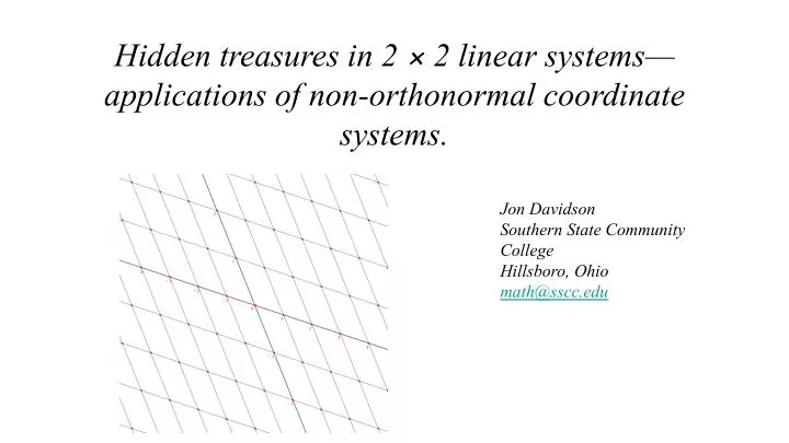
Hidden treasures in 2 × 2 linear systems—applications of non-orthonormal coordinate systems. Jon Davidson Southern State Community College Hillsboro, Ohio math@sscc.edu
For example: What can we learn from an ordinary linear system of two variables? The solution is x = 3, y = 2.
The coefficient matrix, A, describes a vector space in : The matrix form, , for this system is:
The right side of this equation, , is a coordinate, , in this vector space. The matrix form, , for this system is:
Thus we have this equation: The matrix form, , for this system is:
For our example matrix, , the coordinate systems represented by Au = x are as follows: In order to generalize the situation, I find it easier to change the variables to a more convenient system,Au = x,where u represents coordinates (u, v), and x repre-sents coordinates (x, y).
v u
y v x The basis vectors for (u, v) are u = 3i – j v = – 2i + 5j. u
y v x The solution to 3u – 2v = 5 – u + 5v = 7, which is (3, 2) in the (u, v) coordinate system, is found at (5, 7) in the (x, y) coordinate system. u
Each node on the graph represents integer solutions to Au = x. Some observations . . .
y v x u For example, coordinate (14, – 9) in (x, y) shows that (4, – 1) is the solution to this system: 3u – 2v = 14 – u + 5v = – 9
The determinant of A is A “unit square” in the (u, v) coordinate system is a parallel-ogram with area = 13 in the(x, y) coordinate system.
It is a good exercise for students to show that in general, if two adjacent sides of a parallelogram are represented by the vectors and This gives an insight into the Jacobian determinant, used in evaluating multiple integrations.
By adapting our original example this way, 3u – 2v = x – u + 5v = y , it could be used as a coordinate transformation in evaluating a double integral. The Jacobian is:
The unit square can be represented by transforms the unit square to the parallelogram we saw before: In the differential of area, dA = dxdy, can be illustrated by scaling it to a unit square.
Thus the scaling factor of the Jacobian determinant can be visualized in this example. The differential of area in (u, v) is
This substitution turns the original equation into the unit circle: This makes finding the area of this ellipse, easier, provided you know the right substitution: x = 3u – 2v y = – u + 5v Since the Jacobian, the scaling factor, is 13, the area of the ellipse is 13π.
The matrix form for the conic section is which gives interesting avenues for exploration in its own right. Unfortunately, I haven’t figured out a simple way to find a convenient substitution, for the general ellipse,that would turn the equation intoin order to easily determine the area of the ellipse.
But if you could find the suitable x = Tu, it can be shown that Since this is the Jacobian of the coordinate transformation, x = Tu, then it can be determined that the area of the ellipse, The proof is tedious.
For this example, the density is y v x What is the density of the integer nodes coinciding with both (u, v) and (x, y) coordinate systems? u
This coordinate system is generated by the vector space with this ordered basis:
And so the density of the integer nodes is Note that Thus it comes from this linear system: u + 2v = x – u + 4v = y
More intuitive is observing that the area of the “unit” parallelograms is , so this rescales the number of integer nodes by that factor. For the general system, Au = x, provided A is nonsingular and all (u, v) and (x, y) coordinates are integers, the density of integer solutions in at integer nodes is: • An algebraic proof seems tricky for first time linear algebra students.
The more general system, 3u + 2v = x 4u + 3v = y , is based on this vector space: This explains why integer solutions to most systems with a determi-nant of 1 or – 1 are “large” in comparison to the coefficients. For example, consider this system: 3x + 2y = 4 4x + 3y = – 5 The solution is x = 22, y = – 31.
The angle between 3i + 4j and 2i + 3j is about 3.2˚. Because the determinant of the coefficient matrix for 3u + 2v = x 4u + 3v = y is 1, any integer values for the right side, (x, y), will produce integer solutions in (u, v). So the density of the integer nodes is 1. I didn’t attempt to draw this coordinate system, but here are the u and v axes:
If we let be the unit circle in (u, v), then is used to provide a substitution to turn it into (x, y) coordinates: This gives the ellipse For example, how does affect the unit circle? It can be interesting to see how the geometry induced by the transformation A in Au = x affects familiar graphs.
Animating this transformation from circle to ellipse provides a little razzle-dazzle.
Recall this system: 3u + 4v = x 2u + 3v = y
I used this for the transformation matrices: for 0 ≤ t ≤ 1. It is interesting to show that the eigenvectors of are the same as the eigenvectors of A when t ≠ 0. If you have the software to produce animations (I used Maple 15), it might be worth it to work out the procedure with your students as an application of a time parameter.
Here are two more transformations of familiar functions. I find that students are fascinated by such transformations.
Here is the basic cubic, transforms this to:
The graph is Here’s a transformation on v = sin u.
If you’d like a copy of this PowerPoint, please write to me (Jon Davidson) at this address: math@sscc.edu