Download
1 / 99
990 likes | 1.13k Views
Chapter 5 and Appendix A: A-1 through A-5 for now. Geometric Transformations Needed for Animation A Mathematics Chapter. IDEAL BACKGROUND FOR ANIMATION IN GRAPHICS. Need concepts from analytical geometry trigonometry linear algebra vector analysis

E N D
Chapter 5andAppendix A: A-1 through A-5 for now Geometric Transformations Needed for Animation A Mathematics Chapter
IDEAL BACKGROUND FOR ANIMATION IN GRAPHICS • Need concepts from • analytical geometry • trigonometry • linear algebra • vector analysis • Don't need memorized formulas, but intuitive concepts and a few basic formulas that can be understood visually. • We'll take a very pragmatic and utilitarian approach. • Approach will be similar to what we do all the time in computer science---deal with abstract data types
ABSTRACT DATA TYPE (ADT) APPROACH • Initially, don't worry about internal representations of these objects ---i.e. in computer science, we capture concepts using the notions of • a class • objects that are instantiated from the class • Concerned about attributes of class • Concerned about functions defined for the class • (Note: although many of you were introduced to these concepts while learning C++ or Java, the above notions existed before these languages were designed.) • REMEMBER- "class" here is not a C++ class!!!
MOTIVATION FOR ALL THIS • We require a knowledge of vectors and matrices in order to understand animation, in particular: • Motion • Camera placement • How to change between the different coordinate systems • We require a knowledge of the representation of lines, planes, and normals in order to understand • Rendering algorithms • Lighting models
CLASSES- not defined, only described for our setting • scalar Notation: , , • For this class, we will use real numbers. • Define equality: just real number equality • pointNotation: P, Q, R • For this class, we just will use a location in 3D space. • Define equality: identical locations • vector Notation: u, v , wor A, B, C Two attributes: length- a scalar denoted by |v| direction in 3D space Define equality: same length and direction
OPERATIONS ON CLASSES Scalars:Assume the usual real number operations of +, - , *, / Vectors:Defined in 3D space (as well as 2D) scalar times vector -A (i.e. -1A) 2A vector plus vector A + B
u v+u v u+v u VECTOR OPERATIONS Perform addition by the head-to-tail rule. Note that u + v = v + u. To perform subtraction, we need the zero vector- i.e. vector with zero length and no direction. Note that v + (-v) = 0 v -v
VECTOR OPERATIONS To perform subtraction, given u and v, we define u - v to be u + (-v): -v u u v u - v As you might suspect, u - v <> v - u Note: We are NOT "computing"anything with numbers yet. Concentrate on the geometry. For the moment, we are not using any reference system or coordinate system.
(cos , sin ) circle with radius 1 VECTOR OPERATIONS:A bit of trigonometry There are two ways to measure the size of an angle: degrees and radian measure 180o = radians Define u• v, the dot product, to be the scalar |u| |v| cos , 0 <= < and is the angle between u and v We are most often concerned with the sign of u• v as it tells us about the angle between two vectors: u• v > 0 iff 0 <= < 90o u• v = 0 iff = 90o u• v < 0 iff > 90o Some useful trigonometric values: cos sin 0 1 0 /2 0 1 -1 0
(cos , sin ) circle with radius 1 u u v u X v VECTOR OPERATIONS:A bit of trigonometry Define u X v, the cross product, to be the vector whose length is |u||v| sin , 0 <= < with is the angle between u and v and whose direction is given by the right hand rule. Right hand rule: 1. With your right hand, make a gun with your index finger as the barrel, your thumb upright where the hammer would be, and your middle finger extended perpendicular to your palm. 2. Freeze those positions. 3. With u and v joined at the tail, lay the index finger along u and then the middle finger along v. 4. Your thumb will be in the direction of u X v. Note that u X v <> v X u . We are often only interested in the direction of u X v.
VECTOR OPERATIONS Scalar times a vector( more details): Let be a scalar and u a vector. Define uto be the vector with length | ||u| with the direction of u if > 0 the opposite of u if < 0 and, of course, if = 0, the vector is the zero vector or a point. u 2u -3u
P P-Q Q POINT OPERATIONS Many operations are not defined, but a few are and they are useful: 1) We already know a vector + vector CAN be a point. (How?) 2) Given points P and Q, we can defineP-Q as the vector given by 3) Consequently, given a vector v and a point Q there is a unique point P such that P = v + Q We can define addition between a vector and a point as above i.e, given Q and v "anchored" at Q, P is the point at the head of v.
P(2) P(1) v Q = P(0) P(-1) SOME IMPORTANT 3D FORMULAS We won't prove these, but you should understand them intuitively. 1) P() = v + Q Defines all points on a line through Q in the direction of v. Also calleda parametric equation of a line. If the points are in 2D space, the line is in 2D space. If the points are in 3D space, the line is in 3D space. Recall that the line segment between Q and P(1) is defined by choosing 0 <= <= 1
DEFINING A RESTRICTED FORM OF POINT ADDITION Start with P= P() = v + Q Let v = R - Q for points R and Q, Then, P = (R-Q) + Q //substitute R-Q for v = R - Q + Q //distribute = R + (1- )Q //regroup So, we can define a restricted point addition as P = 1R +2Q , when 1 + 2= 1 P() R R-Q Q
P(2) R = P(1) Q = P(0) P(-1) SOME IMPORTANT 3D FORMULAS 2) P() = R + (1- )Q Defines all points on a line through Q and R. We just derived this formula from (1). You should read the derivation, but I will not ask you to reproduce it! Again, to obtain the line segment between R and Q, restrict so that 0 <= <= 1 R-Q
R v Q P u SOME IMPORTANT 3D FORMULAS T(,) = P + (1- )(Q-P) + (1- )(R-P) defines all points on a plane, provided P, Q, and R are not collinear. But, this formula is not as useful as the next one. 3) T(,) = P + u + v , defines all points on the plane as a parametric equation. u and v cannot be parallel vectors
Intuitively,T(,) = P + u + v , defines all points on the plane P + 1.25 u + 1.5v (approximately) R v P u Q
Intuitively,T(,) = P + u + v , defines all points on the plane P + (-0.33) u + -v (approximately) R v Q P u What happens if we restrict and to be between 0 and 1?
v Po u SOME IMPORTANT 3D FORMULAS 4) Another useful equation of a plane is given by (u X v) • (P - P0) = 0 where P is a point on the plane The vector u X v is perpendicular, or orthogonal, to the plane and is called the normal to the plane.
REVIEW • We have defined the following as abstract objects • scalars • points • vectors • And we have defined • dot product • cross product • parametric equation of line • parametric equation of plane • normal to plane • plane equation using the normal
NOTE THAT WE HAVEN'T • Seen how to “compute” anything • Haven't had a coordinate system involved. • These concepts are NOT required in order to visualize what is happening with scalars, points, and vectors. • Now, we have to add a coordinate system, but first we need some basic concepts from analytical geometry.
MATRICES Definition: A matrixis an n X m array of scalars, arranged conceptually in n rows and m columns, where n and m are positive integers. If n = m, we say the matrix is a square matrix. We often refer to a matrix with the notation A = [a(i,j)] where a(i,j) denotes the scalar in the ith row and the jth column We'll use A, B, and C to denote matrices. Note that the text uses the typical mathematical notation where the i and j are subscripts. We'll use this alternative form as it is easier to type and it is more familiar to computer scientists.
MATRIX OPERATIONSDefinitions Scalar-matrix multiplication: A = [ a(i,j)] Matrix-matrix addition: A and B are both n X m C = A + B = [a(i,j) + b(i,j)] Matrix-matrix multiplication: A is n X r and B is r X m r C = AB = [c(i,j)] where c(i,j) = a(i,k) b(k,j) k=1 Examples...
MATRIX OPERATIONSExamples Scalar-matrix multiplication: A = [ a(i,j)] 3 -1 15 -5 5 7 2 = 35 10 -1 6 -5 30 Matrix-matrix addition: A and B are both n X m C = A + B = [a(i,j) + b(i,j)] 3 -1 5 2 8 1 7 2 + 3 -1 = 10 1 -1 6 4 0 3 6
MATRIX OPERATIONSExamples Matrix-matrix multiplication: A is n X r and B is r X m r C = AB = [c(i,j)] where c(i,j) = a(i,k) b(k,j) k=1 For example, 3 -1 1 2 1 -1 0 5 3 -1 c(2,3)= a(2,1)b(1,3) + 1 2 3 1 0 -2 = 7 4 1 -5 a(2,2)b(2,3)= 0 1 3 1 0 -2 1*1 + 2*0 = 1 must be the same Note that the following is undefined: 1 2 1 -1 3 -1 because a 2 X 4 matrix can't be 3 1 0 -2 1 2 multiplied by a 3 X 2 matrix. 0 1 A 4 X m matrix is required.
MATRIX OPERATIONSDefinitions (Continued) Transpose: A is n X m. Its transpose, AT, is the m X n matrix with the rows and columns reversed. Inverse: Assume A is a square matrix, i.e. n X n. The identity matrix, In has 1s down the diagonal and 0s elsewhere The inverse A-1 does not always exist. If it does, then A-1 A = A A-1 = I There are many algorithms for finding A-1, but we won't worry about them as the software will find the values. However, given a matrix A and another matrix B, we can check whether or not B is the inverse of A by computing AB and BA and seeing that AB = BA = In More examples ...
MATRIX OPERATIONSExamples Transpose: A is n X m. Its transpose, AT, is the m X n matrix with the rows and columns reversed. 1 2 1 4T = 1 3 3 1 0 5 2 1 1 0 4 5 Inverse: Assume A is a square matrix, i.e. n X n. If A-1 exists, then A-1 A = A A-1 = I 1 0-1 1 0 2 3 = -2/3 1/3 because 1 0 1 0 1 0 1 0 1 0 2 3 -2/3 1/3 = -2/3 1/3 2 3 = 0 1 THIS DOES NOT SHOW HOW TO FIND THE INVERSE!
BASIS Definition: Any 3 vectors v1, v2, and v3 that satisfy the two properties: 1) (linearly independence) 1v1 + 2v2 + 3v3 = 0 if and only if 1 = 2 = 3 = 0 2) (spanning) Any vector v in the space can be represented uniquely as the linear combination of the basis vectors, i.e. v = 1v1 + 2v2 + 3v3 is called a basis for the space. FACT: In 2D space, any basis needs 2 vectors. In 3D space, any basis needs 3 vectors.
BASIS Example: 1) Linear independence: the zero vector u + v = 0 can happen only if and are 0 u v Any vector w can be written as a linear combination of u and v: w w = u + v for some and u w v
BASIS- Don't think the basis vectors must be perpendicular to each other Example: 2) Linear independence: a point u + v = 0 can happen only if and are 0 u v w The vector w can be written as a linear combination of u and v: w u w = u + v for some and v
FRAMES Definition: A frame is a point P0 and a basis v1, v2, and v3 in 3D space. We can specify a frame as (v1, v2, v3, P0) Given a frame, any point P can be represented in the frame as P = 1v1 + 2v2 + 3v3 + P0 and any vector v can be written as v = β1v1 + β2v2 + β3v3 + 0·P0 In the previous slides, the P0 is just the point where the vectors are joined--- i.e. what we often call the origin (or the reference point) of the coordinate system. We will now use matrices to represent some of these concepts.
HOMOGENEOUS COORDINATES In many textbooks, a vector is associated with a point (x, y, z) where the x, y, and z represent the coordinates in the standard coordinate system. This only works if we assume the frame we are using has the point (0,0,0) as the origin and the vector is positioned at the origin: This causes confusion as the vector from (1,1,1) to (2,3,4) is the same vector as the one from (0,0,0) to (1,2,3) because the vectors have the same length and their directions are the same.
HOMOGENEOUS COORDINATES • In graphics, • we wish to keep points and vectors as separate entities • we wish to maintain frame information. • We use homogeneous coordinates to represent points and vectors. • A homogeneous coordinate is a 4D column or row matrix • (This can be defined in projective geometry, but we don't need the definition here- only the properties of a homogeneous coordinate--- it acts like any other matrix.)
HOMOGENEOUS COORDINATE REPRESENTATION OF A 3D POINT We assume a frame is specified,(v1, v2, v3, P0), and, consequently any point P can be written uniquely as P = 1v1 + 2v2 + 3v3 + P0 If we agree to define 1 • P = P, we can write this formally as the matrix product: P=[ 1 2 3 1]v1. v2 v3 P0 So, we choose to represents a point P in a frame (v1, v2, v3, P0) as column matrix: [ 1 2 3 1]T
HOMOGENEOUS COORDINATE REPRESENTATION OF A 3D POINT We assume a frame is specified,(v1, v2, v3, P0), and, consequently any vector v can be written uniquely as v = β1v1 + β2v2 + β3v3 + 0·P0 If we agree to define 0• P0 = 0, we can write this formally as the matrix product: v=[ β1β2β3 0]v1 . v2 v3 P0 So, we choose to represents a point v in a frame (v1, v2, v3, P0) as column matrix: [ β1β2β3 0]T
SO, POINTS AND VECTORS HAVE SIMILAR, BUT DIFFERENT REPRESENTATIONS! Note the simplicity and similarity of the representations, given some frame: • 2 3 4 1]T is a point in the frame. • 1 4 5 0]T is a vector in the frame. Only the 4th component, the 1 or the 0, tells us whether we have a point or a vector.
WHY WORRY ABOUT ALL OF THIS? We will define our objects in a physical frame. The camera can be expressed in this frame, but it is more useful to switch to a camera frame where the origin is at the center of a projection. Moreover, it will be most useful if we can define our objects in a frame that is handy to use for computational purposes and then SWITCH frames to a more natural one.
MOTION OR ANIMATION IS JUST A FRAME CHANGE. You can think of motion as holding the frame still and moving the object or holding the object still and moving the frame!
CHANGING FRAMES Problem: Given a frame (v1, v2, v3, P0) and another frame (u1, u2, u3, Q0) , we need an easy way to transfer the representation of a point or a vector in one frame to the appropriate representation of the point or the vector in the other frame. Recall: In the frame (v1, v2, v3, P0), any point P can be written as 1v1 + 2v2 + 3v3 + P0 and any vector v can be written as 1v1 + 2v2 + 3v3
CHANGING FRAME ALGORITHM(A VERY, VERY IMPORTANT ALGORITHM!)We will revisit this so don’t sweat the details now Given a frame X = (v1, v2, v3, P0) and another frame Y= (u1, u2, u3, Q0) 1) Represent the basis vectors ui and the point Q0 of Y in the frame X: u1 = 11v1 + 12v2 + 13v3 + 0•P0 where γij is the scalar u2 = 21v1 + 22v2 + 23v3 + 0•P0 in the ith row u3 = 31v1 + 32v2 + 33v3 + 0•P0 and jthcolumn. Q0 = 41v1 + 42v2 + 43v3 + 1•P0
2) Represent the equations as a matrix equation. u1 v1 u2 v2 u3 = M v3 where M is the matrix Q0 P0 11 12 13 0 21 22 23 0 31 32 33 0 41 42 43 1 This 4 X 4 matrix M is called the frame change matrix. Note that it is unique.
3)We can use the matrix M to compute for any point or vector its new representation in frame Y or conversely. Let a be either a point or vector in X. Then a = MT b (convert Y frame to X frame) or b= (MT)-1 a (convert X frame to Y frame) where b is the corresponding point or vector in Y. Thus, M allows us to move back and forth between frames!
THE DERIVATION OF THE FORMULAS u1 v1 11 12 13 0 u2 v2 21 22 23 0 u3 = M v3 where M is the matrix 31 32 33 0 Q0 P0 41 42 43 1 Let a and b be homogeneous coordinate representations of either a point or a vector in X = (v1, v2, v3, P0) and Y= (u1, u2, u3, Q0) respectively. Then, bTu1 = bTM v1 = aTv1 u2 v2 v2 bTM = aT (bTM)T = (aT)T u3 v3 v3 Q0 P0 P0 a = MTb (formula to convert Y to X) (MT)-1 a = (MT)-1 MTb = In b b = (MT)-1 a (formula to convert X to Y)
y x z FRAMES IN OPENGL • We've seen that the representation of points and vectors are tied to frames. • OpenGL maintains two frames • Camera frame • World frame • Initially, the two frames are the same with the following orientation: Camera is pointing along the negative z axis. This is a right-handed system.
y y x x z z BUT, WE WISH TO BE ABLE TO MOVE OBJECTS (OR MOVE FRAMES) Hint: Imagine you are sitting so your eye is looking in the negative z direction towards the origin (reference point) in each frame. Where do you see the cube? To your left? In front of you? Does it appear when you switch frames that the cube has moved? new frame original frame Although each activity is the same, it is often easier to think that you are moving objects. BUT, either visualization is fine!
THE USUAL SCENARIO IN OPENGL • Define objects around the origin in the default setting. • We want the viewing conditions to be such that the camera sees only those objects we wish it to see. • So, we need to move • 1) the camera away from the objects or • 2) the objects away from the camera. • Or, equivalently, we move • 1)' the camera frame relative to the world frame or • 2)' the world frame relative to the camera frame. • Normally, we view the camera as fixed and move the objects.
THE IMPORTANT MODEL-VIEW MATRIX • This is the 4 X 4 frame change matrix that is required to transform between camera frame representations and world frame representations. • We can change the matrix by loading the necessary 16 scalars using glLoadMatrix. • But, computing the 16 scalars is not an easy task as we have seen. • It is easier, to equivalently move objects, using affine transformations.
AFFINE TRANSFORMATIONS • A transformationis a function that maps a point (or vector) into another point (or vector). • An affine transformationis a transformation that maps lines to lines. Why are affine transformations "nice"? • We can define a polygon using only points and • the line segments joining the points. • To move the polygon, if we use affine transformations, • we only must map the points defining thepolygon • as the edges will be mapped to edges! We can model many objects with polygons--- and should--- for the above reason in many cases.
AFFINE TRANSFORMATIONS • VERY IMPORTANT FACT: Any affine transformation can be obtained by applying, in sequence, transformations of the form • Translate • Scale • Rotate- 3 different types in 3D space • So, to move an object all we have to do is determine the sequence of transformations we want using the 3 types of affine transformations above.