Download
1 / 20
200 likes | 366 Views
SPATIAL PATTERN ANALYSIS PROGRAM FOR QUANTIFYING LANDSCAPE STRUCTURE. Fragmentation involves changes in landscape composition, structure, and function across scales. An important topic in conservation biology and ecology to better understand the cause and the consequences.

E N D
SPATIAL PATTERN ANALYSIS PROGRAM FOR QUANTIFYING LANDSCAPE STRUCTURE Fragmentation involves changes in landscape composition, structure, and function across scales. An important topic in conservation biology and ecology to better understand the cause and the consequences. ** The paper recommended (McGarigal and Cushman 2002) summarizes the fragmentation studies with the most recent and richest references on the topic.
** Among the 134 papers (studies) reviewed Edge, Patch, Patch-Landscape, Landscape 8% 39% 19% 22% ** Mensurative (>75%, differ in time or space) and Manipulative (pre- post-treatment in a controlled manner while keep all other factors constant, 7 features and hard to implement) No single solution for complex Q, but GIS…(e.g. FRAGSTATS) method is recommended.
EM means many different things to many different people, but there is a general agreement that it does involve making dec. in a LS context, Consequently, LS analysis is becoming an integral part of EM. A necessary component of LS analysis is the quantification of LS structure. There are basically two versions of FRAGSTATS: vector and raster. It has been improved from 2.0 in early 1990s (ftp ftp.fsl.orst.edu) to currently 3.3 with much better computer interface (http://www.umass.edu/landeco/research/fragstats/downloads/fragstats_downloads.html).
Usage: The command line contains as many as 18 parameters but most are set optional or default. We discuss several key inputs here: *.exe in-file out-file cellsize edge_dist data_type rows cols, … Input format: Several but basically as image or ascii files (background value -999).
Output files: root name with extension of *.patch (13), *.class (39), *.land (45), and *.full (some of indices are N/A). Output formats differ slightly between V and R, but the calculation concept for the same indices are similar to each other. Case study: Fragmentation and edge effects on landscape-level soil respiration in Chequamegon D. Zheng, J. Chen, J.M. LeMoine, and E.S. Euskirchen
Clearcuts across the landscape 1972 2001
Tsedge = Tscc – proportion * (Tscc – Tsforest) Tscc > Tsforest Tsedge = Tscc + proportion * (Tsforest - Tscc) Tscc < Tsforest
(MH) 0.2974 * e0.0635*Ts, r2 = 0.73 (CC) 0.2594 * e0.0513*Ts, r2 = 0.67 (YF) 0.3195 * e0.0715*Ts, r2 = 0.65 (JP) 0.3235 * e0.0514*Ts, r2 = 0.45 (RP) 0.3059 * e0.0611*Ts, r2 = 0.55 Euskirchen et al. 2003
∆SRR=1.36*∆AWMPFD+0.076 r2=0.495 ∆ AWMPFD (2001-1972, unitless)
∆SRR=0.0063*∆ED+0.0353 r2=0.422 ∆ ED (2001-1972, m.ha-1)
∆SRR=0.0097*∆PRO+0.0835 r2=0.420 ∆ Proportion of clearcut (2001-1972, %)
SRRedge = 0.0787 + 1.221 * AWMPFD(2001-1972) r2 = 0.491 AWMPFD = Area-Weighted Mean Patch Fractal Dimension.
Potential significance of model application: 1) changes in SRR associated with fragmentation and edge effects are difficult to measure for any areas at the landscape level or larger; 2) remote sensing images at various spatial resolutions are available for mapping land cover changes over time and AEI caused by clearcuts can be further identified or calculated across the landscapes; 3) the landscapes used in this study for model development cover a wide range in term of clearcut proportions to entire landscapes, from <1% to >20%. Weaknesses: 1) Forest dominated LS; 2) not water limited conditions only.
CONCLUSION 1) Both land-use change and edge effects associated with clearcuts can affect field season landscape SRR but at different magnitudes. Lc changes in the 16 subs (72-01) on SRR ranged from –2.6-4% with an average of 0.5%; edge = 0.03% in 72 & 0.16% in 2001, on average). Convergent process vs. spread-out process in edges. 2) Edge effects on SRR deserve more attention, yet are complex and at relatively smaller magnitude compared to T and LC. Edge effects on SRR global carbon balance are not clear and need more studies. SoilM is more important in a dry environment. Larger edge effects on SRR are expected in areas with more frequent and intensive disturbances (roads and ownership). 3) Changes in SRR were strongly related to class-level fragmentation indices but not LS-level indices (Fragstats is one of useful tools for such analyses). 4) This study developed a simple approach to examine changes in SRR caused by edge effects in landscapes that are difficult to measure from Fragm. indices that are relatively easy to calculate.
TNPP = 0.46 * PPT – 7.4 * TMEAN + 218.3 * NDVI – 52.5 * AET + 332.5 r2 = 0.883 TNPP = 0.386 * PPT + 219.9 * NDVI – 9.4 * TMAX + 0.7 * CO2 – 43.5 r2 = 0.869 TNPP in g C/m2/yr, PPT in mm, T in 0C, NDVI unitless (0-1), AET in mm/yr, and CO2 in ppm.