Download
1 / 23
230 likes | 328 Views
Compression Domain Volume Rendering. Jean Shneider and Rudiger Westermann Computer graphics and Visualization group Technical university Munich. Motivation. Need to deal with data of increasing size: Large-scale Multi-dimensional Multi-parameter Increasing problems: Compression

E N D
Compression Domain Volume Rendering Jean Shneider and Rudiger Westermann Computer graphics and Visualization group Technical university Munich
Motivation Need to deal with data of increasing size: • Large-scale • Multi-dimensional • Multi-parameter Increasing problems: • Compression • Representation • Rendering We will adress all three problems!
Talk Outline The Approach – Vector Quantization Quality and speed • Hierachical encoding • PCA-Split • Progressive encoding of time-resolved data Multi-dimensional data • Vectors of arbitrary length Rendering from compressed data • GPU-based decoding and rendering • Per-fragment evaluation • Interactive framerates
Talk Outline The Application – Volume Rendering • Large-scale volumetric data sets • Time-varying sequences 1.4 GB / 20 fps 16 MB / 14 fps 0.78 MB / 11 fps 70 MB / 24 fps 256^3, rendered from compressed 256^3x89 timesteps
Input mapping Encoder in=E(Xn) Xn Codebook C with codewords Decoder in X‘n=C(in) Output mapping Vector Quantization - data fitting 4D vectors Introduces quantization error • VQ assymetric, encoding expensive, decoding free => exploit this!
Vector Quantization LBG-Algorithm • Linde, Buzo and Gray 1980 • Iterative refinement of a previous Codebook • Sensitive to quality of first Codebook • Usually computationally expensive Speed-Up possible (and necessary) • Partial searches • Fast searches • Better initial Codebook (i.e. PCA-Splits) LBG-Algorithm can be fast!
Vector Quantization The PCA-Split • Lensch et.al. 2001 – BRDF Compression • Covariance analysis to find optimal splitting plane • Cut a cluster of input vectors in two by this plane. • Plane is given by centroid of current set and largest Eigenvector (= normal) of the Auto-Covariance Matrix
Vector Quantization LBG as PCA post-processing • Increases fidelity • Leads to stable Voronoi-Regions • Only a few steps are necessary • Great speed-up compared to LBG only! A series of LBG steps, codebook from last slide
Example Full-color confocal microscopy scan, 5122x32xRGB 32D vectors, 1MB 4D vectors, 2MB Original, 32MB
Hierarchical Vector Quantization full Laplace Decomposition ½ res 3 freq bands - that is a combination of a smoothening and a difference filter. This results in a three level hierarchy of volumes ¼ res
43 dim. VQ 23 dim. VQ Direct Copy Hierarchical Vector Quantization 256 64D vectors blocks 4^3 scalar samples together into one vector Codebook 256 8D vectors
Hierarchical Vector Quantization Output: • One RGB Index-Volume • Two Codebooks RGB Index-Volume 3D Texture Codebooks 2D -Textures
Example Visible Human (Male), RGB slice 2048x1216 Compression took 10.0 seconds, PSNR = 34.72dB Compression ration - 25:1 Original (7.1MB) Compressed (285KB)
Timings Reference System: P4 2.8GHz, 1GB memory VHP Slice, 2048x1216 RGB 10.0 sec Engine 2562x128 CT-Scan 19.0 sec Skull 2563 CT-Scan 50.6 sec Vortex Sequence, 1283x100 13 (5) min Shockwave Sequence, 2563x89 29 (13) min
Decoding process in flatland Rendering GPU-based decoding • Indices stored in 3D RGB-texture (3/64th original size) • Decode index per block dependent fetch • Decode adress per block 43 adress texture
Rendering Render 3D index and adress texture • Nearest neighbor interpolation for both • GL_REPEAT for adress texture Per-fragment decoding • Decode detail components and dependent fetch • Add the details to average component (Red channel) • Lookup result in 1D RGB transfer function Problem: Complex fragment shader slows down rendering
Rendering Solution:Deferred Fragment Processing Avoid decoding in empty regions. „Empty“ means: a) -Transfer function maps 0 0. • Check on CPU • Switch between two possible rendering modes b) Average value is 0 (Red channel) • Check in a first, simple fragment program • Fragment‘s depth value is set accordingly • Second pass: discard (early Z-Test) or render fragment • Full decoding only performed in second pass
2562x128 Engine CT Scan 19.0 seconds, PSNR = 36.17dB (P4 2.8GHz) Compressed (402KB) – 12 fps Original (8MB) – 19 fps
2563 Skull CT Scan 50.6 seconds, PSNR = 35.35dB (P4 2.8GHz) Original (16MB) – 14 fps Compressed (780KB) – 11 fps
Time-resolved Sequences Exploit temporal coherences during compression: • Group of Frames (GOF) First frame in a GOF: • PCA-Split followed by LBG-Refinement Other frames: • LBG-refinement of last Index-Volume and Codebook Result: • Great speed-up (factor 2 to 3) • Very large GOFs possible (64+ frames) • Virtually same fidelity as frame-by-frame
1283x100 Vortex-Simulation 5 minutes, PSNR = 34.43dB (P4 2.8 GHz) Original (200MB) - 28 fps Compressed (11MB) - 16 fps
2563x89 Shockwave-Sequence 13 minutes, PSNR = 51.36dB (P4 2.8 GHz) Original (1.4GB) - 20 fps Compressed (70MB) - 24 fps
Conclusions • Compression ratios of approx. 20:1 • Interactive rendering possible • Easy random access to each frame • Wide variety of data sets handled Currently only nearest neighbor interpolation • Mainly limited by performance / instruction count. • Tri-linear interpolation can be done on newer GPUs!