Download
1 / 10
100 likes | 233 Views
Statistically motivated quantifiers GUHA matrices/searches can be seen from a statistical point of view , too. We may ask ‘Is the coincidence of two predicates (x) and (x) just random or is there some

E N D
Statistically motivated quantifiers GUHA matrices/searches can be seen from a statistical point of view, too. We may ask ‘Is the coincidence of two predicates (x) and (x) just random or is there some statistically justified dependence between them’? For example, it is custom to use the 2 test to compare observed and expected values; a genetic experiment might hypothesise that the next generation of plants will exhibit a certain set of colours. By comparing the observed results with the expected ones, we can decide whether our original hypothesis is valid. We will study two statistically motivated quantifiers in details and mention several others Fisher quantifier, 0 < 0.5. Fisher quantifier corresponds to the test of hypothesis Probability((x)|(x)) > Probability((x)|(x)) with significance . For example, our data may concern health and smoking. Let v((x)) = TRUE mean ‘x is a smoker’ and v((x))) = TRUE mean ‘x has cancer. If an output of a GUHA procedure is (x) 0.05(x), we accept the hypothesis ‘Smoking causes cancer’ and doing so there is a 0.05 probability that we make a mistake. More precisely, a Fisher quantifier (on the level , 0 < 0.5) is defined such that, for any model M, v(((x) (x))= TRUE iff ad > bc and I
Theorem 9. Fisher quantifier is associational. Proof. Consider models M0, M1, M2, M3, M4 such that and (i) vM0(((x) (x))= TRUE. We should show that (ii) vM1(((x) (x))= TRUE, (iii) vM2(((x) (x))= TRUE, (iv) vM3(((x) (x))= TRUE, (v) vM4(((x) (x))= TRUE. However, since Fisher quantifiers are invariant under interchanging b and c and under interchanging a and d, we have to prove (ii) and (iii) only. Assume (i). Then First we notice bc ad +d, which holds true by assumption.
Second, we notice that, for each i = 0,…,min{b,c} Therefore Trivially (a+1)d > bc. Therefore (ii) holds. Next consider the model M2 and the value 1° Let b c. First notice that which holds true by assumption. Second, notice that, for all i = 0,…,b-1 we have Obviously, the last inequality is true. We may now estimate B:
2° Let c < b [i.e. c b-1]. Again and, for each i = 0,…,c, Trivially, ad > (b-1)c. This completes the proof. Theorem 10. and are sound rules of inference for Fisher quantifiers Proof. The claim becomes obvious as soon as we realise that, for any model M, interchanging ( and ) or ( and , and ) has no effect on the values
Lehman proved in 1959 that Fisher test is the most powerful in the class of unbiased tests of the null hypothesis 0 and the alternative hypothesis > 0. On the other hand, the computation of the Fisher test for larger m is complicated, the complexity of computation increasing rapidly. For this practical reason, another test, the 2 test is widely used. This test is only asymptotical, but the approximation is rather good for reasonable cardinalities (a, b, c, d 5, m d 20). We will see that Fisher quantifier and 2 quantifier have similar properties. For the exact definition of the 2 quantifiers, recall the following: let a continuous one- dimensional distribution function D(x) be given. For each [0,1], the value D-1() is called the -quantile of D. The 2 quantifier (on the level ) is defined such that v((x) (x)) = TRUE iff ad > bc and I where is the (1-) quantile of the 2-distribution function. In practice, an 2-association rule (x) (x)) corresponds to a test (on the level ) of the null hypothesis of independence of (x) and(x) against the alternative one of the positive dependence. Theorem 10. 2-quantifiers are associational. Proof. The 2-quantifiers are invariant under interchanging b and c and under inter- changing a and d. Thus, it is enough to show that if (i) vM0(((x) (x))= TRUE, then (ii) vM1(((x) (x))= TRUE (iii) vM2(((x) (x))= TRUE, too, where
First we realise that, for any numbers A, B, x, y greater than 0, it holds that Thus, in particular Since b2c2 = bcbc abcd, we have b2c2(r + k + 1) abcd(r + k + 1). Thus, to prove (*) it is sufficient to prove Substituting r = a + b, k = a + c results (by Maple)
We have now proved the inequality Therefore we have Trivially (a+1)d > bc holds. We conclude We summarise: if vM0(((x) (x))= TRUE, then vM1(((x) (x))= TRUE. Next consider an inequality (*) is equivalent to the following inequality: The right hand side of (**) is obviously 1. Moreover, since the left hand side of (**) is 1. Therefore (**) holds and, hence, (*) holds, too. Trivially ad > (b-1)c. We have shown: if vM0(((x) (x))= TRUE, then vM2(((x) (x))= TRUE, too. This completes the proof. Theorem 11. For 2-quantifiers and are sound rules of inference. Proof. The claim is obvious as, for any model M, interchanging ( and ) or ( and , and ) has no effect on the values
Exercises. Some more statistically motivated quantifiers. Show that the following quantifiers are implicational. 23. Lower critical implication!p, Base, where 0 < p 1, 0 < 0.5 and Base > 0. v((x) !p, Base(x)) = TRUE iff An association rule (x) !p, Base(x) corresponds to a test (on the level of ) of a null hypothesis H0: P(Suc|Ant) p against the alternative one H1: P(Suc|Ant) > p. If the association rule (x) !p, Base(x) is true in data matrix M then the alternative hypothesis is accepted. 24. Upper critical implication?p, Base, where 0 < p 1, 0 < 0.5 and Base > 0. v((x) ?p, Base(x)) = TRUE iff An association rule (x) ?p, Base(x) corresponds to a test (on the level of ) of a null hypothesis H0: P(Suc|Ant) p against the alternative one H1: P(Suc|Ant) < p. If the association rule (x) ?p, Base(x) is true in data matrix M then the alternative hypothesis is accepted.
Show that the following quantifiers are associational. 24. Double lower critical implication!p, Base, 0 < p 1, 0 < 0.5 and Base > 0. v((x) !p, Base(x)) = TRUE iff 25. Double upper critical implication?p, Base, 0 < p 1, 0 < 0.5 and Base > 0. v((x) ?p, Base(x)) = TRUE iff
Show that the following quantifiers are associational. 26. Lower critical equivalence!p, Base, 0 < p 1, 0 < 0.5 and Base > 0. v((x) !p, Base(x)) = TRUE iff 27. Upper critical implication?p, Base, 0 < p 1, 0 < 0.5 and Base > 0. v((x) ?p, Base(x)) = TRUE iff