Download
1 / 44
440 likes | 549 Views
Learning Cycle-Linear Hybrid Automata for Excitable Cells Radu Grosu SUNY at Stony Brook. Joint work with Sayan Mitra and Pei Ye. Motivation. Hybrid automata: an increasingly popular formalism for approximating systems with nonlinear dynamics

E N D
Learning Cycle-Linear Hybrid Automata for Excitable CellsRadu GrosuSUNY at Stony Brook Joint work with Sayan Mitra and Pei Ye
Motivation • Hybrid automata: an increasingly popular formalism for approximating systems with nonlinear dynamics • modes: encodevarious regimes of the continuous dynamics • transitions: express the switching logic between the regimes • Excitable cells: neuronal, cardiac and muscular cells • Biologic transistors whose nonlinear dynamics is used to • Amplify/propagate an electrical signal (action potential AP)
Motivation • Excitable cells (EC) are intrinsically hybrid in nature: • Transmembrane ion fluxesand AP vary continuously, yet • Transition from resting to excited states is all-or-nothing • ECs modeled with nonlinear differential equations: • Invaluable asset to reveal local interactions • Very complex: tens of state vars and hundreds of parameters • Hardly amenable to formal analysis and control
Project Goals • Learn linear HA modeling EC behavior (AP): • Measurements readily available in large amounts • Analyze HA to reveal properties of ECs: • Setting up new experiments for ECs may take months • Synthesize controllers for ECs from HA: • Higher abstraction of HA simplifies the task • Validate in-vitro the EC controllers: • Cells grown on chips provided with sensors and actuators
Impact • 1 million deaths annually: • caused by cardiovascular disease in US alone, or • more than 40% of all deaths. • 25% of these are victims of ventricular fibrillation: • many small/out-of-phase contractions caused by spiral waves • Epilepsy is a brain disease with similar cause: • Induction and breakup of electricalspiral waves.
Mathematical Models • Hodgkin-Huxley (HH) model (Nobel price): • Membrane potential forsquid giant axon • Developed in 1952. Framework for the following models • Luo-Rudy (LRd) model: • Model forcardiac cells of guinea pig • Developed in 1991. Much more complicated. • Neo-Natal Rat (NNR) model: • Being developed at Stony Brook by Emilia Entcheva • In-vitro validation framework. Very complicated, too.
K+ Na+ Outside C Na K L Inside Active Membrane Conductances vary w.r.t. time and membrane potential
Ist Outside INa IK IL IC gNa gK gL C V VNa VK VL Inside Currents in an Active Membrane
Ist Outside INa IK IL IC gNa gK gL C V VNa VK VL Inside Currents in an Active Membrane
Ist Outside INa IK IL IC gNa gK gL C V VNa VK VL Inside Currents in an Active Membrane
Ist Outside INa IK IL IC gNa gK gL C V VNa VK VL Inside Currents in an Active Membrane
Ist Outside INa IK IL IC gNa gK gL C V VNa VK VL Inside Currents in an Active Membrane
vn Frequency Response APD90: AP > 10% APmDI90: AP < 10% APmBCL:APD + DI
vn Frequency Response APD90: AP > 10% APmDI90: AP < 10% APmBCL:APD + DI S1S2 Protocol: (i) obtainstable S1;(ii) deliverS2 with shorter DI
Frequency Response APD90: AP > 10% APmDI90: AP < 10% APmBCL:APD + DI S1S2 Protocol: (i) obtainstable S1;(ii) deliverS2 with shorter DI Restitution curve: plot APD90/DI90 relation for different BCLs
Learning Luo-Rudi • Training set: for simplicity25APsgenerated from the LRd • BCL1 + DI2: from 160ms to 400 ms in 10ms intervals • Stimulus: stepwith amplitude-80A/cm2,duration0.6ms • Error margin: within 2mV of the Luo-Rudi model • Test set: 25APsfrom 165ms to 405 ms in 10ms intervals
Stimulated Roadmap: One AP
Stimulated Roadmap: Linear HA for One AP
Stimulated Roadmap: Linear HA for One AP
Stimulated Roadmap: Cycle-Linear HA for All APs
Stimulated Roadmap: Cycle-Linear HA for All APs
Finding Segmentation Pts Null Pts: discrete 1st Order deriv. Infl. Pts: discrete 2nd Order deriv. Seg. Pts: Null Pts and Infl. Pts Segments: between Seg. Pts Problem:too many Infl. Pts Problem:too many segments?
Finding Segmentation Pts Null Pts: discrete 1st Order deriv. Infl. Pts: discrete 2nd Order deriv. Seg. Pts: Null Pts and Infl. Pts Segments: Between Seg. Pts Problem:too many Infl. Pts Problem:too many segments? • Solution: use a low-pass filter • Moving average and spline LPF: not satisfactory • Designed our own: remove pts within trains of inflection points • Solution: ignore two inflection points
Finding Segmentation Pts Problem:some inflection points disappear in certain regimes Solution:ignore (based on range) additional inflection points
Finding Segmentation Pts • Problem:removing points does not preserve desired accuracy • Solution: align and move up/down inflection points • - Confirmed by higher resolution samples
Exponential Fitting • Exponential fitting: Typical strategy • Fix bi: do linear regression on ai • Fix ai: nonlin. regr. in bi ~> linear regr.in bi via Taylor exp. • Geometric requirements: curvesegments are • Convex,concave or both • Upwards or downwards • Consequences: • Solutions: might require at least two exponentials • Coefficients ai andbi: positive/negative or real/complex • Modified Prony’s method: only one that worked well
Stimulated Linear HA for One AP
Finding CLHA Coefficients Solution:apply mProny once again on each of the 25 points
Stimulated Cycle-Linear HA for All APs
Stimulated Cycle-Linear HA for All APs
Frequency Response on Test Set AP on test set:still within the accepted error margin Restitution on test set:much better than we had before Frequency response: the best we know for approximate models
I2 I1 b2 b1 –b2 x1 C V b1 x2 Biological Meaning of x1 and x2 Two gates: with constant conductances distributed as above
Outlook: Modeling Entire Range • Modes 1&2: require 3 state variables (Na, K, Ca) • Shape changes dramatically: modes are sidestepped • Input:consider different shapes and intensities
Outlook: Analysis and Control • Safety properties: • How to specify: what kind of temporal/spatial properties? • How to verify: what kind of reachability analysis? • Liveness properties: • Stability analysis:switching speed and stability/bifurcation • Controllability: • Design centralized (distributed) controllers:from CLHA • Control task: diffuse spirals and ventricular fibrillation