Download

1 / 20
200 likes | 366 Views
CGS 3763: Operating System Concepts Spring 2006 Uniprocessor Scheduling – Part 2. Instructor : Mark Llewellyn markl@cs.ucf.edu CSB 242, 823-2790 http://www.cs.ucf.edu/courses/cgs3763/spr2006. School of Electrical Engineering and Computer Science University of Central Florida.

E N D
CGS 3763: Operating System Concepts Spring 2006 Uniprocessor Scheduling – Part 2 Instructor : Mark Llewellyn markl@cs.ucf.edu CSB 242, 823-2790 http://www.cs.ucf.edu/courses/cgs3763/spr2006 School of Electrical Engineering and Computer Science University of Central Florida
Characteristics of Various Scheduling Protocols See notes FCFS = first come first served SPN = shortest process next SRT = shortest remaining time HRRN = highest response ration next
Process Scheduling Example As we examine the various scheduling protocols we’ll use this set of processes as a running example. We can think of these as batch jobs with the service time representing the total execution time required. Alternatively, we can think of these as ongoing processes that require alternate use of the processor and I/O in repetitive fashion. In this case, the service time represents the processor time required in one cycle. In either case, in terms of a queuing model, this quantity corresponds to the service time.
Shortest Process Nest (SPN) is another approach to reduce the bias in favor of long processes that is inherent with FCFS. SPN is nonpreemptive. The process with the shortest expected processing time is selected next by the scheduler. Thus, a short process job will jump to the head of the queue passing longer jobs. Shortest Process Next (SPN)
Shortest Process Next • Waiting times: A = 0, B = 1, C = 7, D = 9, E = 1 • Average waiting time = (0 + 1 + 7 + 9 + 1)/5 = 3.6 • Turnaround times (Tr): A = 3, B = 7, C = 11, D= 14, E = 3 • Average turnaround time = (3 + 7 + 11 + 14 + 3)/5 = 38/5 = 7.6 • Tr/Ts: A = 3/3 = 1, B = 7/6 = 1.17, C = 11/4 = 2.75, D = 14/5 = 2.8, E = 3/2 = 1.5 • Average Tr/Ts = (1 + 1.17 + 2.75 + 2.8 + 1.5)/5 = 9.22/5 = 1.84 Notice that Process E receives service much sooner under SPN than it did under FCFS.
In terms of response time, overall performance has improved under this protocol. However, the variability of response times has also increased, especially for longer processes, and thus predictability of longer processes is reduced. One difficulty with the SPN protocol is the need to know or accurately predict the required processing time for each process. If estimated time for process not correct, the operating system may abort it. Possibility of starvation for longer processes occurs if there is a steady supply of short processes. Not favored for time-sharing or transaction processing environments due to the lack of preemption. Shortest Process Next
The Shortest Remaining Time (SRT) protocol is a preemptive version of SPN. In SRT, the scheduler always chooses the process that has the shortest expected remaining processing time. When a new process joins the ready queue, it may have a shorter remaining time than the currently running process. If this occurs, the scheduler may preempt the current process when the new process arrives. As with SPN, the SRT scheduler must have an estimate of the processing time in order to perform the selection funciton. Again, there is the possibility of starvation for longer processes. Shortest Remaining Time (SRT)
SRT does not have the bias in favor of long processes that we saw with FCFS. Unlike RR, no additional interrupts are generated, which reduces the overhead. On the other hand, elapsed service time must be recorded which contributes to overhead. SRT typically gives superior turnaround time performance when compared to SRP, because a short job is given immediate preference to a running longer job. Note in the example on the next page that the three shortest processes (A, C, and E) all receive immediate service, which produces a normalized turnaround time of 1.0 for each. Shortest Remaining Time (SRT)
Shortest Remaining Time • Waiting times: A = 0, B = 7, C = 0, D = 9, E = 0 • Average waiting time = (0 + 7 + 0 + 9 + 0)/5 = 16/5 = 3.2 • Turnaround times (Tr): A = 3, B = 13, C = 4, D= 14, E = 2 • Average turnaround time = (3 + 13 + 4 + 14 + 2)/5 = 36/5 = 7.2 • Tr/Ts: A = 3/3 = 1, B = 13/6 = 2.17, C = 4/4 = 1, D = 14/5 = 2.8, E = 2/2 = 1 • Average Tr/Ts = (1 + 2.17 + 1 + 2.8 + 1)/5 = 7.97/5 = 1.59
Highest Response Ration Next (HRRN) uses the normalized turnaround time, which is the ratio Tr/Ts. HRRN attempts to minimize the average of this ratio over all processes. In general, it is not possible to know in advance what the exact service time will be, but it can be approximated, based either on past history or some input from the user or a configuration manager. The scheduler’s decision is now determined as follows: when the current process completes or is blocked, choose the ready process with the greatest value of this ratio. Highest Response Ratio Next (HRRN)
This approach is attractive because it accounts for the age of the process. While shorter jobs are favored (a smaller denominator results in a larger ratio), aging without service increases the ratio (since Tr gets larger) so that a longer process will eventually get past competing shorter jobs. Highest Response Ratio Next (HRRN)
Highest Response Ratio Next (HRRN) time spent waiting + expected service time expected service time • Waiting times: A = 0, B = 1, C = 5, D = 9, E = 5 • Average waiting time = (0 + 1 + 5 + 9 + 5)/5 = 19/5 = 3.8 • Turnaround times (Tr): A = 3, B = 7, C = 9, D= 14, E = 7 • Average turnaround time = (3 + 7 + 9 + 14 + 7)/5 = 40/5 = 8.0 • Tr/Ts: A = 3/3 = 1, B = 7/6 = 1.17, C = 9/4 = 2.25, D = 14/5 = 2.8, E = 7/2 = 3.5 • Average Tr/Ts = (1 + 1.17 + 2.25 + 2.8 + 3.5)/5 = 10.72/5 = 2.14
If the scheduler has no way of knowing or estimating with any degree of accuracy the relative length of the various processes it may schedule, then none of SPN, SRT, or HRRN can be used. Another technique for establishing a preference for shorter jobs is to penalize jobs that have been running longer. In other words, if the scheduler cannot focus on the time remaining to execute, then let it focus on the time spent in execution so far. The mechanism for doing this is as follows: Scheduling is done on a preemptive basis (assuming some time quantum), and a dynamic priority mechanism is applied. When a process first enters the system Feedback Techniques (FB)
Scheduling is done on a preemptive basis (assuming some time quantum), and a dynamic priority mechanism is applied. When a process first enters the system, it is placed in RQ0 (see diagram on next page). After its first preemption, when it returns to the ready state, it is placed in RQ1 (next lowest priority). Each subsequent time that it is preempted, it is demoted to the next lower priority queue. Within each priority queue, except for the lowest level queue, a simple FCFS mechanism is used. Once in the lowest level queue a process cannot have a lower priority so it is repeatedly returned to this queue until it completes execution. So this queue is handled in round-robin fashion. Feedback Techniques
Short processes will complete quickly, without moving very far down the hierarchy of ready queues. A longer process will gradually drift down the priority queue hierarchy. Thus newer shorter processes are favored over older longer processes. There are a number of variations on the feedback protocol. In the simplest case, preemption is performed in the same fashion as for round-robin, i.e., at periodic intervals. (This is shown in the example on page 18 for a time quantum of 1.) Feedback Techniques
There is a problem with this simple mechanism however, in that the turnaround time of longer processes can grow at an alarming rate. Starvation is possible, if new jobs are entering the system frequently. To compensate for this, the preemption times can be varying depending on the queue (feedback level) in the following fashion: A process scheduled from queue RQ0 is allowed to execute for 1 time quantum and then is preempted. A process scheduled from queue RQ1 is allowed to execute for 2 time quanta. In general, a process scheduled from queue RQi is allowed to execute for 2i time quanta. Feedback Techniques
Feedback Techniques Feedback Time quantum = 1 for all queue levels Waiting times: A = 1, B = 12, C = 8, D = 8, E = 1 Average waiting time = (0 + 12 + 8 + 8 + 1)/5 = 30/5 = 6.0 Turnaround times (Tr): A = 4, B = 18, C = 12, D= 13, E = 3 Average turnaround time = (4 + 18 + 12 + 13 + 3)/5 = 50/5 = 10.0 Tr/Ts: A = 4/3 = 1.33, B = 18/6 = 3, C = 12/4 = 3, D = 13/5 = 2.6, E = 3/2 = 1.5 Average Tr/Ts = (1.33 + 3 + 3 + 2.6 + 1.5)/5 = 11.43/5 = 2.29
Feedback Techniques Feedback Time quantum = 2i for all queue levels Waiting times: A = 1, B = 9, C = 10, D = 9, E = 4 Average waiting time = (1 + 9 + 10 + 9 + 4)/5 = 33/5 = 6.6 Turnaround times (Tr): A = 4, B = 15, C = 14, D= 14, E = 6 Average turnaround time = (4 + 15 + 14 + 14 + 6)/5 = 53/5 = 10.6 Tr/Ts: A = 4/3 = 1.33, B = 15/6 = 2.5, C = 14/4 = 3.5, D = 14/5 = 2.8, E = 6/2 = 3 Average Tr/Ts = (1.33 + 2.5 + 3.5 + 2.8 + 3)/5 = 13.13/5 = 2.63