Download
1 / 30
300 likes | 395 Views
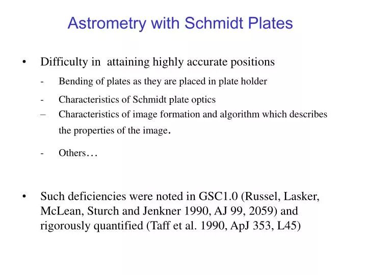
Astrometry with Schmidt Plates. Difficulty in attaining highly accurate positions Bending of plates as they are placed in plate holder Characteristics of Schmidt plate optics Characteristics of image formation and algorithm which describes the properties of the image . Others …

E N D
Astrometry with Schmidt Plates • Difficulty in attaining highly accurate positions • Bending of plates as they are placed in plate holder • Characteristics of Schmidt plate optics • Characteristics of image formation and algorithm which describes the properties of the image. • Others… • Such deficiencies were noted in GSC1.0 (Russel, Lasker, McLean, Sturch and Jenkner 1990, AJ 99, 2059) and rigorously quantified (Taff et al. 1990, ApJ 353, L45)
Plates 0019 and 04JJ From Morrison,Roeser, McLean, Bucciarelli and Lasker 2001, AJ 121,1752 (GSC1.2)
Sub–plate method (Taff 1989, AJ 98, 1912; Taff Lattanzi and Bucciarelli, 1990, ApJ 358,359 ) Collocation method (Fresneau 1978, AJ 83, 406; Lattanzi and Bucciarelli 1991, A&A 250, 565; Bucciarelli Lattanzi and Taff 1993, ApJS 84, 91) Mask method (Taff Lattanzi and Bucciarelli, 1990, ApJ 358,359 ) Local filters (Morrison, Smart and Taff 1998, MNRAS 296, 66; Roeser, Bastian and Kuzmin 1995, IAU Coll. 148, ASP Conf. Ser. Vol 84) Successful Reduction Techniques
Comparisons to external catalogs Compare residuals from overlapping plates Residuals (from 1 & 2) vs. magnitude Characterization of Systematic Errors • Position-only dependent errors • Magnitude and Position dependent errors. • Global: common to a set of plates. • Local: vary from plate to plate. • Methods to Detect them:
External Reference Catalogs • ACT • AC2000 + TYCHO • All sky catalog • 958,758 objects • TYCHO 2 • 2.5 million objects • Position accuracy 10 – 100 mas • Proper motion accuracy 1 – 3mas • Limiting in magnitude ~ 11.5
NPM • 300,000 stars • - 23 to 90 ( 72% of northern sky) • 8 < B < 18 • SPM • 25 to –40 but not in the galactic plane. • 321,608 stars • 5 < V < 18.5 • 2MASS • Strip scans (currently 40% of sky) • 8200 stars/square degree • Complete to roughly V= 18 • UCAC1 • Current catalog sky coverage south of –15 deg. • Limiting in magnitude R = 16 • 2000 stars/square degree • 20 mas for 10 to 14, 70 mas for 15 to limits External Faint Reference Catalogs
GSCII Astrometric Pipeline • Input parameters: measured X,Y values and and of plate center, observation conditions. • Output variables: and of every object on the plate • Plate_solution • Pre-correct for differential refraction • Equidistant projection • Quadratic plate model • Note: Resulting positions have the well known position and magnitude dependent errors: 0.8 to 1.4 arc seconds near the plate edges. • Astrometric Mask • Using all available plates for a survey determines corrections common to a set of plates.
Modelled Third Order Effects Equidistant Projection Differential Refraction • Zr – Z0 = A tan(Z0) + + B tan3(Z0 ) + ….. • A ~ 60”.3 • B ~ 0.”067
Residuals from Overlapping Plates 3105 star pairs (every 5th star plotted) Mean residual: 0.37 Mean residual: 0.53
Astrometric Mask • Mask is created: • Create a grid of closely spaced points.(40x40). • Spacing of grid points needs to be smaller than scale of systematics. • Around each grid point find all the reference stars contained in the filter and determine the , corrections. • Mask is stored • Mask is applied: • Find the closest grid point and near by N grid points. • Correction determined by weighting based on distance of object from grid points.
Vector Mask of Averaged Residuals Plate residuals stacked onto the Schmidt plate frame SPlates /N~500 Consequence of : a. Physical deformation of the Schmidt plate. b. Characteristics of Schmidt plate optics. c. Characteristics of centroider and image formation. d. a,b and c result in effects which are not understood from a engineering/physics standpoint to be adequately represented in the plate model. Swirl Pattern of systematic errors varying across the plate (worse at the edges 1" ) Average number of stars/bin = 109
XJ Mask XP Mask
XS Mask ER Mask
XV Mask GR Mask
XI Mask: Palomar IR IS Mask: UK Schmidt IR
Residuals from Overlapping Plates Overlapping Schmidt Plates comparing the positions of the same star imaged on 2 plates. 3105 stars pairs (every 5 star plotted). Before mask applied After mask applied Mean xi residual: 0.37 arc seconds Mean eta residual: 0.53 arc seconds Mean xi residual: 0.20 arc seconds Mean eta residual: 0.37 arc seconds
Reducing Systematics on Individual Plates Filter Method: Transforms the plate-based system to a system defined by a dense and homogenous reference catalog. Corrections to each image on the plate are found by: • Draw a circle around every image. • Find all the reference stars in circle. • For each match determine , . • Corrections to the central object: weighted average of all , . Central Image Matched Reference Star
Residuals from Overlapping Plates Plate Solution Mask Filter 86110 stars 1/10th of stars plotted Plate Solution: residual: 0.40 0.58 residual: 0.12 0.43 Mask: residual: 0.40 0.26 residual: 0.11 0.25 Filter: residual: 0.26 0.22 residual: 0.10 0.20
Magnitude Dependent Systematics MagnitudeEquation • Experience with GSC I Global magnitude equation (coma-like) (Morrison, Roeser, Lasker, Smart and Taff 1996, AJ 111, 1405). • Plate-to-Plate positional magnitude- dependent errors (guiding) (Lu, Platais, Girard, Kozhurina-Platais, van Altena 1998, IAU Symp. 179, p.384)
Magnitude Dependent Systematics Detect and quantify • Overlapping plates • a. Same bandpass • b. Different bandpasses (full plate overlaps) • c. A set of co-added pairs (for the same geometric overlap pattern). • Faint reference catalog for comparison • Limited relevance to GSC2.2 because of the method of selecting position – chose the one closest to plate center reduced magnitude dependence
Preliminary testing on GSCII database • -Using 55 GSC II plates (OOP files) compared GSC II positions with those in the SPM. • Residuals showed a magnitude dependence in the positions. • Increase in the amplitude of the residuals starting at 11.5 and steadily increasing with magnitude.
SPM - GSC II database magnitude test Test study: 55 plates
Summary of GSCII Astrometric Calibrations • Plate Solution: equidistant projection, differential refraction, least-squares fit • Astrometric mask: reduces global position-only systematic errors • Magnitude correction: reduces magnitude-dependent systematic errors (currently in testing). • Filter method : reduces local small-scale systematic errors remaining across individual plates (currently in testing).
GSC2.2 Positional Accuracy • Plate Solution + Astrometric Mask: • Averaged over all plates: accuracy ~ 0.25” positional • Plate-to-Plate variations exist up to 0.2-0.3 arcseconds per coordinate
” GSC2 – SPM (STARS) (*cos) = (_____) () = (……..) 1740 48662 10704 47842 74190 mF
__ ” GSC2 – SPM (STARS) ________ (*cos) = (_____) ____ () = (……..) 1740 48662 74190 10704 47842 mF
” GSC2 – NPM (STARS) 99 (*cos) = (_____) () = (……..) 9495 4107 51886 19153 mF
__ ” GSC2 – NPM (STARS) ________ (*cos) = (_____) 99 ____ () = (……..) 9495 4107 51886 19153 mF
CATALOGS USED FOR COMPARISON WITH GSC2 CATALOGS TOTAL OBJECTS % OF OUTLIERS >10” NPM STARS 148363 0.20 SPM STARS 285235 0.76 SUB-CATALOGS GOOD OBJS. (*) RETAINED OBJS. IN 3 % OBJECTS GSC2S - NPMS 87239 85202 97.56 GSC2S - SPMS 189171 183448 96.97 (*) Are the objs. with |*cos| and | |<10” and 0 < mF < 24