Download
1 / 24
400 likes | 1.03k Views
Topic 7 - Fourier Transforms. Department of Physics and Astronomy. DIGITAL IMAGE PROCESSING Course 3624. Professor Bob Warwick. 7.1 Review of The Fourier Transform. Many DIP techniques rely on the application of an image transform of which the Fourier Transform is the most popular.

E N D
Topic 7 - Fourier Transforms Department of Physics and Astronomy DIGITAL IMAGE PROCESSING Course 3624 Professor Bob Warwick
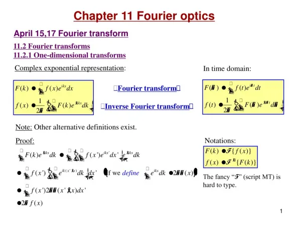
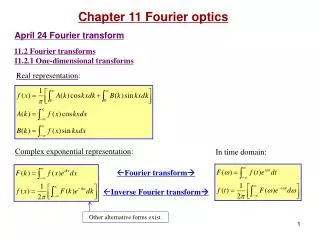
7.1 Review of The Fourier Transform • Many DIP techniques rely on the application of an image transform of which the Fourier Transform is the most popular. • The Fourier domain provides very important insight into the information content of the data. Outline of this Topic 7.1 Introduction to the Fourier Transform (FT) 7.2 The Discrete Fourier Transform (DFT) 7.3 The Properties of the DFT 7.4 Computation of the DFT (via the FFT) 7.1 Introduction to the FT In 1-d, assuming continuous variables: Fourier Transform Pair may often be real, whereas F(u) is generally complex, ie
Spatial Frequency The spatial frequency of this signal would be: with units of either: cycles per m(physical space) cycles per pixel (image space) F(u) is a two-side function of u (i.e. extends to +ve and –ve frequencies) If f(x) is real:
Fourier Transform of a Gaussian • Notes: • The Inverse Relationship – narrow function in the spatial domain results in a wide function in the Fourier Domain. • In this case F(u) is not complex ie
A Table of FT Pairs RECTANGULAR FUNCTION GAUSSIAN FUNCTION DELTA FUNCTION COSINE FUNCTION SINE FUNCTION SHAH FUNCTION
The 2-D Fourier Transform y v x u Example: The "Box Car" Function
More on Convolution Integrals Example: Convolution of a Shah Function with a Rectangular Function The CONVOLUTION THEOREM: the Fourier Transform of the product of two functions equals the convolution of the Fourier transforms of the individual functions.
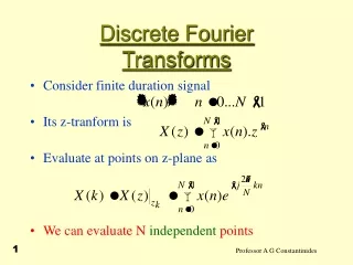
Consider a 1-d sampled dataset of dimension N: 7.2 The Discrete Fourier Transform (DFT) We need to evaluate F(u) on a grid of N points (in u space). A good choice for the spacing is Δu=1/X (=1 cycle across the full extent of the image)
The DFT continued Finally we set , we redistribute the normalization term and drop the dashes: EXAMPLE: Determine the DFT of a 4-point dataset with input values: f0 = 1 f1 = 1 f2 = 0 f3 = 0 |Fu| X X X X X X X X X X X X -4 -3 -2 -1 0 1 2 3 4 5 6 7 u Why the periodicity?
7.3 Some Properties of the DFT (a) SAMPLING THEORY Assume F(u) is zero outside range -w<u<w S(u) is a Shah Function with spacing Δu=1/Δx In the Fourier domain we have the convolution S(u)*F(u) Input data stream (continuous variables) Represent sampling by a comb of delta functions s(x) [a Shah Function] The sampled version of f(x) can be represented by s(x)f(x) This explains the periodic nature of the DFT ie it repeats at a rate (in u) of 1/Δx However, if the bandwidth of the input signal w is too high , such that w > 1/2Δx, then the result will be The overlap of the repeating functions results in information loss ALIASING
Some Properties of the DFT cont. • SHANNON’S SAMPLING THEOREM • To avoid information loss it is necessary to sample a signal at a rate equivalent to at least twice the maximum frequency component present in the signal. • That is we need w < 1/2Δx, where 1/2Δx is known as the Nyquist frequency. To avoid aliasing sample at a higher rate (or alternatively filter the input data stream to remove signals above the Nyquist frequency) ✖ ✔ The process to recover the original data stream!
Some Properties of the DFT cont. (c) CHARACTER OF THE DFT Example: 1-d 8-point transform. |Fu| fx 0 1 2 3 4 5 6 7 x 0 1 2 3 4 5 6 7 x N=8 N=8 • The 2-D DFT • The Optical Transform • A trick to shift the (u,v) origin from the top left corner to the centre of the Fuv image is to multiply the input image by alternate 1’s and -1’s before computing the DFT i.e.
In DIP applications we need to compute the 2-d DFT 7.4 Computation of the DFT The “separability” property of the 2-d transform leads to a simplification: Hence, the 2-d DFT reduces to the computation of a series of 1-d transforms. y v v 2 1 fxy Fxv Fuv x x u Step 1 involves N 1-d transforms along the rows of the original image (x N scaling) Step 2 involves N 1-d transforms down the columns of the intermediate image In total we require 2N 1-d transforms, each of which involves N x N complex multiplies and adds ie N4 2N3 calculations
A Fortran FFT Routine Re-ordering Successive doubling
Calculating the Inverse Fourier Transform If we take the complex conjugate of the inverse transform and scale by 1/N: • To calculate the Inverse Transform with a software procedure that computes the 1-d “forward” transform: • Convert Fu Fu* • (ii) Apply the forward transform • (iii) Scale the result by N • (iv) Convert fx* fx
Example of a 2-d DFT calculation fxy (-1)x+y |Fuv | log |Fuv |
And the Inverse …. (-1)x+y Ignoring the amplitude! Ignoring the phase!
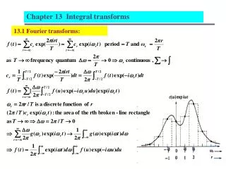
Example of a 2-d DFT log |Fuv| Richard Alan Peters II
Magnitude-only Reconstruction Phase-only Reconstruction