Download
1 / 24
270 likes | 425 Views
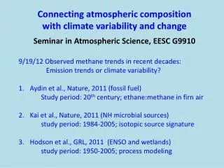
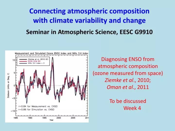
Connecting atmospheric composition with climate variability and change Seminar in Atmospheric Science, EESC G9910. Diagnosing ENSO from atmospheric composition (ozone measured from space) Ziemke et al ., 2010; Oman et al ., 2011 To be discussed Week 4. Course Information.

E N D
Connecting atmospheric composition with climate variability and change Seminar in Atmospheric Science, EESC G9910 Diagnosing ENSO from atmospheric composition (ozone measured from space) Ziemke et al., 2010; Oman et al., 2011 To be discussed Week 4
Course Information • Two motivating questions: • How does climate variability (and change) influence distributions of trace species in the troposphere? • How do changes in trace species alter climate? Email me by Monday Sept 10: a) to sign up for presentation: amfiore @ ldeo.columbia.edu b) Credit options: 1 point (discussion only) 2 points (discussion + presentation) Weekly readings at www.ldeo.columbia.edu/~amfiore/eescG9910.html
Today’s Outline • Overview of composition-climate interactions • Intro to key concepts • a. Units of atmospheric composition • b. Budgets / Lifetimes • c. Radiative Forcing
Big Issues in Atmospheric Chemistry Point source Urban smog Ozone layer Visibility Disasters Climate Regional smog Biogeochemical cycles Acid rain GLOBAL > 1000 km LOCAL < 100 km REGIONAL 100-1000 km Daniel Jacob
From Brasseur & Jacob, Ch2, draft chapter Jan 2011 version; Text in prep
Air pollutants affect climate; changes in climate affect global atmospheric chemistry (and regional air pollution) Greenhouse gases absorb infrared radiation • Smaller droplet size • clouds last longer • increase albedo • less precipitation T T T Black carbon Sulfate organic carbon Aerosols interact with sunlight “direct” + “indirect” effects O3 H2O NMVOCs CO, CH4 + + OH NOx atmospheric cleanser pollutant sources Surface of the Earth A.M. Fiore
Climate (change) affects chemistry (and air quality) (1) Transport / mixing (e.g., distribution of trace species) Exchange with stratosphere strong mixing sources (2) Emissions (biogenic, lightning NOx, fires) VOCs (3) Chemistry responds to changes in temperature, humidity NMVOCs CO, CH4 O3 NOx OH + + H2O PAN tropopause Planetary boundary layer A.M. Fiore
remains constant when air density changes e robust measure of atmospheric composition • Air also contains variable H2O vapor (10-6-10-2 mol mol-1) and aerosol particles 1.1 Mixing ratio or mole fraction CX[mol mol-1] Trace gases Trace gas concentration units: 1 ppmv = 1 µmol mol-1 = 1x10⁻⁶ mol mol-1 1 ppbv = 1 nmol mol-1 = 1x10⁻⁹ mol mol-1 1 pptv = 1 pmol mol-1 = 1x10-12 mol mol-1 Daniel Jacob
1.2 Number density nX[molecules cm-3] • Proper measure for • reaction rates • optical properties of atmosphere Proper measure for absorption or scattering of radiation by atmosphere nXand CXare relatedby the ideal gas law: na = air density Av = Avogadro’s number P = pressure R = Gas constant T = temperature MX= molecular mass of X Also define the mass concentration (g cm-3): Daniel Jacob
ATMOSPHERIC BUDGET TERMS GLOBAL SOURCE: emissions, in situ production (Tg yr-1) well-known for some (well-documented) synthetic gases GLOBAL SINK: chemical destruction, photolysis, deposition (Tg yr-1) ATMOSPHERIC BURDEN: total mass (Tg) integrated over the atmosphere Well known (measurements) for long-lived (well-mixed) gases Poorly constrained for short-lived species TREND: difference between sources and sinks (Tg yr-1) More detail: TAR 4.1.3
Recent trends in well-mixed GHGs http://www.esrl.noaa.gov/gmd/aggi/
More than half of global methane emissions are influenced by human activities ~300 Tg CH4 yr-1 Anthropogenic [EDGAR 3.2 Fast-Track 2000; Olivier et al., 2005] ~200 Tg CH4 yr-1 Biogenic sources [Wang et al., 2004] >25% uncertainty in total emissions Clathrates? Melting permafrost? PLANTS? 60-240 Keppler et al., 2006 85 Sanderson et al., 2006 10-60 Kirschbaum et al., 2006 0-46 Ferretti et al., 2006 BIOMASS BURNING + BIOFUEL 30 ANIMALS 90 WETLANDS 180 LANDFILLS + WASTEWATER 50 GAS + OIL 60 COAL 30 TERMITES 20 RICE 40 GLOBAL METHANE SOURCES (Tg CH4 yr-1) A.M. Fiore
Lifetimes Atmospheric Lifetime: Amount of time to replace burden (turnover time) t (yr) = burden (Tg) / mean global sink (Tg yr-1) for a gas in steady-state (unchanging burden; sources = sinks Convenient scale factor: (1) constant emissions (Tg/yr) steady-state burden (Tg) (2) emission pulse (Tg) time integrated burden of that pulse (Tg/yr) Perturbation (e-folding) Time – can differ from the atmospheric steady-state lifetime only equal to atmospheric lifetime for gases with constant chemical lifetime (e.g., Rn, radioactive decay) Chemical feedbacks (e.g., CH4: more CH4, longer CH4 lifetime; N2O: more N2O, shorter lifetime Lifetimes can vary spatially and temporally -- species with lifetimes shorter than mixing time scales (< 1 year) (TAR 4.1.4)
TIME SCALES FOR HORIZONTAL TRANSPORT(TROPOSPHERE) 1-2 months 2 weeks 1-2 months 1 year c/o Daniel Jacob
TYPICAL TIME SCALES FOR VERTICAL MIXING tropopause (10 km) 10 years 5 km 1 month 1 week 2 km planetary boundary layer 1 day 0 km c/o Daniel Jacob
Radiative Forcing (RF): A convenient metric for comparing climate responsesto various forcing agents RF = Change in net (down-up) irradiance (radiative flux) at the tropopause due to a perturbation to an atmospheric constituent • Why is this convenient/useful ? • First order estimate, best for LLGHGs • Relatively easy to calculate (as opposed to climate response) • Related to global mean equilibrium T change at surface: Climate sensitivity parameter Global, annual mean change in surface T in response to RF (equilibrium) DTs = l * RF
Solar blackbody fn. Earth’s “effective” blackbody fn. CFCs Clouds, Aerosols active throughout spectra Methane Nitrous oxide Oxygen; Ozone Carbon dioxide Water vapor c/o V. Ramaswamy uv vis near-ir longwave
IR Transmission/Absorption in/near atmospheric window From Jan 2012 version Ch 5 of Brasseur & Jacob textbook in prep
Radiative Forcing: Analytical expressions for Well-mixed GHGs From IPCC TAR CH6, Table 6.2 http://www.esrl.noaa.gov/gmd/aggi/
Radiative Forcing (RF): comparison of calculation methodologies Figure 2.2, WG1 IPCC AR-4 Chapter 2, Section 2.2
Radiative forcing of climate (1750 to present):Important contributions from non-CO2 species IPCC, 2007
Global Warming Potentials • Radiative forcing does not account for different atmospheric lifetimes of forcing agents • GWP attempts to account for this by comparing the integrated RF over a specified period (e.g. 100 years) from a unit mass pulse emission, relative to CO2.
The atmosphere seen from space WHAT IS THE ATMOSPHERE? • Gaesous envelope surrounding the Earth • Mixture of gases, also contains suspended solid and liquid particles (aerosols) • Aerosol = dispersed condensed phase suspended in a gas Aerosols are the “visible” components of the atmosphere California fire plumes Dust off West Africa Pollution off U.S. east coast Daniel Jacob
ATMOSPHERIC GASES ARE “VISIBLE” TOO…IF YOU LOOK IN THE UV OR IR Nitrogen dioxide (NO2 ) observed by satellite in the UV Daniel Jacob