Download
1 / 22
220 likes | 314 Views
An Efficient Algorithm for Scheduling Instructions with Deadline Constraints on ILP Machines. Wu Hui Joxan Jaffar School of Computing National University of Singapore. What is an ILP machine?. Multiple functional units of different types.

E N D
An Efficient Algorithm for Scheduling Instructions with Deadline Constraints on ILP Machines Wu Hui Joxan Jaffar School of Computing National University of Singapore
What is an ILP machine? • Multiple functional units of different types. • Issue an instruction every machine cycle on each functional unit. • Multiple instructions executed in parallel. • Latencies exist between instructions. • Two categories: Superscalar and VLIW (Very Long Instruction Word). • Typical Example: Intel Itanium processor (http://developer.intel.com/design/ia64/microarch_ovw/index.htm)
What is the problem? • Given a problem instance P: a set of n UET instructions in a basic block with the following constraints: • precedence-latency constraints: DAG G = (V, E, W), where each latency lij -1, • deadline constraints: individual pre-assigned deadlines, and • m functional units with p different types, • compute a feasible schedule which satisfies all constraints whenever one exists, or a valid schedule with minimum lateness if no feasible schedule exists.
v1 [4] v2 [4] v3 [4] FU1 1 0 1 FU2 1 0 0 0 v4[5] v5 [5] v6 [5] v7 [5] 0 0 0 0 0 v8 [6] v9 [6] v10 [6] v11 [6] v12 [6] Example 1. A problem instance P with two functional units of different types. Table 1. A feasible schedule for P.
What does our algorithm achieve? Our scheduling algorithm computes a feasible schedule whenever one exists for any problem instance of the following special cases. 1) Arbitrary DAG, latencies of 0 and two functional units of different types. 2) Monotone interval graph, latencies -1 and multiple functional units of different types. 3) In-forest, equal latencies and multiple functional units of different types.
In the case that there is no feasible schedule, our algorithm computes a schedule with minimum lateness for all the above special cases. • Furthermore, by setting all deadlines to a constant, our algorithm will compute a schedule with minimum completion time for • any instance of the above special cases and • any instance of the special case of out-forest, equal latencies and multiple functional units of different types.
v2 v3 v1 v1 v4 v5 v2 v3 v6 v4 v5 v6 An in-tree. An out-tree v1 v2 2 3 2 3 v3 v4 v5 -1 1 2 1 4 v6 v7 A monotone interval graph.
What is the Time Complexity ? • Given the transitive closure of the precedence graph, • O(ne+nd) for the general model, where d is the maximum latency. • O(min{ne, de}+nd) if no latency of -1 exists. • O(n2) if for each instruction the latencies between it and all its immediate successors are equal. • Transitive closure can be computed in O(min(ne, n2.367)) time.
What has been done in the past? • Palem and Simon’s algorithm on identical processors [ACM TOPLAS, 1993]. • Wu, Joxan and Yap’s algorithm on identical processors [PACT 2000]. • Berstein, Rodeh and Gertner’s work on two processors of different types [IEEE TOC, 1989].
What are the contributions of our work? • Propose an efficient polynomial algorithm which solves several special cases for each of which no polynomial algorithm was known before. • Present the first approximation ratio, i.e. for any greedy algorithm, the length of any schedule computed never exceeds p+1, where p is the number of types of functional units.
What are the main ideas of our algorithm? • Compute the lmax(vi)-successor-tree-consistent deadline for each instruction vi, where lmax(vi)is the maximum latency between vi and all its immediate successors. • Compute a schedule by using list scheduling, where the priority of each instruction is its successor-tree-consistent deadline and a smaller number implies higher priority.
What is the lmax(vi)-successor-tree-consistentdeadline? • For each sink instruction, its lmax(vi)-successor-tree-consistentdeadline d´i is equal to its pre-assigned deadline. • For a non-sink instruction vi, d´i is the upper bound on its latest completion time in any feasible schedule for the relaxed problem instance P(i).
What is P(i)? • P(i) consists of a set V(i)={vi} Succ(vi) of instructions with following new constraints. • Precedence-latency constraints: The lmax(vi)-successor-tree of vi. • Deadline constraints: The deadline of each instruction vj in Succ(vi) is its lmax(vj)-successor-tree-consistentdeadline and the deadline of vi is its pre-assigned deadline.
What is the k-successor-tree of vi ? • Given a weighted graph G=(V, E, W), an integer k and vi V, the k-successor-tree of vi is a subgraph G= (V, E, W), where • V ={vi} {vj: vj Succ(vi)}, • E={(vi, vj): vj Succ(vi)} and • each edge weight l´ij in W is defined as follows. • 1) In the case that k= -1, if l+ij = -1, then l´ij = -1; otherwise l´ij = 0. • 2) In the case that k -1, if l+ij < k, then l´ij = l+ij; otherwise, l´ij = k.
v1 v2 4 2 1 -1 1 v3 v4 v5 1 0 1 v7 v8 v6 Figure 1: The precedence-latency constraints. v2 4 4 1 2 -1 1 v3 v6 v4 v7 v5 v8 Figure 2: The 4-successor tree of v2.
How to compute lmax(vi)-successor-tree-consistent deadline for vi ? • Key idea: Backward Scheduling • At any time t, among all ready instructions, an instruction vk with the largest latency in P(i) is chosen and scheduled as late as possible on a functional unit of the same type. In case of ties, among all instructions with the same latency, an instruction with the latest deadline is chosen. • A schedule computed by backward scheduling is called a backward schedule.
FU1 FU2 v1 [2] 3 3 1 2 -1 1 v2[5] v3[6] v4[5] v5 [3] v6[4] v7[3] Example 2: A relaxed problem instance P(1). Table 2. A backward schedule for P(1).
Scheduling Algorithm • repeat • choose an instruction vi satisfying that 1) its lmax(vi)-successor-tree-consistent deadline d´i has not been computed; and 2) either vi is a sink or the successor-tree-consistent deadlines of all its successors have been computed; • if vi is a sink then d´i = di; • else • { if vi has only one immediate successor vj and lij -1 • then d´i = min{di, dj - lij - 1}; • else • { compute a backward schedule b for P(i); • d´i = min{di, min{b(vj) - lij : vj Succ(vi) }}; • } } • until the successor-tree-consistent deadlines of all instructions have been computed; • use list scheduling to compute a schedule for P, where the priority of each instruction vi is d´i and a smaller number implies higher priority;
v1 [4, ?] v2 [4] v3 [4] FU1 1 0 1 FU2 1 0 0 0 v4[5, 4] v5 [5, 5] v6 [5, 5] v7 [5, 5] 0 0 0 0 0 v8 [6, 6] v9 [6, 6] v10 [6, 6] v11 [6, 6] v12 [6, 6] Example 1. A problem instance P with two functional units of different types. V1[4] 0 0 1 1 1 1 1 V4 [4] V5 [5] V 6[5] V8 [6] V9 [6] V10 [6] V11 [6] Figure 4: The relaxed problem P(1).
Table 3: A backward schedule b for Succ(v1). Since min{b(vj) - l1j : vj Succ(v1)}= 2, the lmax(v1)-successor-tree-consistent deadline of v1is min{d1, 2}= min{4, 2}= 2.
v1 [4, 2] v2 [4, 3] v3 [4, 3] FU1 1 0 1 FU2 1 0 0 0 v4[5, 4] v5 [5, 5] v6 [5, 5] v7 [5, 5] 0 0 0 0 0 v8 [6, 6] v9 [6, 6] v10 [6, 6] v11 [6, 6] v12 [6, 6] Example 1. A problem instance P with two functional units of different types. Table 3. A feasible schedule computed by list scheduling.
Conclusion • K-successor-tree-consistency: • A general technique for instruction scheduling problem. • Approximating precedence-latency constraints by using priorities which are k-successor-tree consistent. • Successfully used to solve several open instruction scheduling problems such as two processor scheduling with equal execution times and release time-deadline constraints. • Open Problem: • What is the tight worst-case approximation ratio of our algorithm (Conjecture: Lours / Lopt = 4/3)?