Download
1 / 34
340 likes | 426 Views
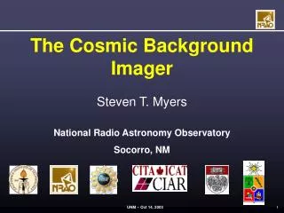
Polarization Results from the Cosmic Background Imager. Steven T. Myers. Continued…. Jonathan Sievers (CITA) Cosmo 04. The CBI Collaboration.

E N D
Polarization Results from the Cosmic Background Imager Steven T. Myers Continued… Jonathan Sievers (CITA) Cosmo 04
The CBI Collaboration Caltech Team: Tony Readhead (Principal Investigator), John Cartwright, Clive Dickinson, Alison Farmer, Russ Keeney, Brian Mason, Steve Miller, Steve Padin (Project Scientist), Tim Pearson, Walter Schaal, Martin Shepherd, Jonathan Sievers, Pat Udomprasert, John Yamasaki. Operations in Chile: Pablo Altamirano, Ricardo Bustos, Cristobal Achermann, Tomislav Vucina, Juan Pablo Jacob, José Cortes, Wilson Araya. Collaborators: Dick Bond (CITA), Leonardo Bronfman (University of Chile), John Carlstrom (University of Chicago), Simon Casassus (University of Chile), Carlo Contaldi (CITA), Nils Halverson (University of California, Berkeley), Bill Holzapfel (University of California, Berkeley), Marshall Joy (NASA's Marshall Space Flight Center), John Kovac (University of Chicago), Erik Leitch (University of Chicago), Jorge May (University of Chile), Steven Myers (National Radio Astronomy Observatory), Angel Otarola (European Southern Observatory), Ue-Li Pen (CITA), Dmitry Pogosyan (University of Alberta), Simon Prunet (Institut d'Astrophysique de Paris), Clem Pryke (University of Chicago). The CBI Project is a collaboration between the California Institute of Technology, the Canadian Institute for Theoretical Astrophysics, the National Radio Astronomy Observatory, the University of Chicago, and the Universidad de Chile. The project has been supported by funds from the National Science Foundation, the California Institute of Technology, Maxine and Ronald Linde, Cecil and Sally Drinkward, Barbara and Stanley Rawn Jr., the Kavli Institute,and the Canadian Institute for Advanced Research.
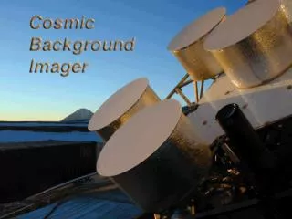
The Instrument • 13 90-cm Cassegrain antennas • 78 baselines • 6-meter platform • Baselines 1m – 5.51m • 10 1 GHz channels 26-36 GHz • HEMT amplifiers (NRAO) • Cryogenic 6K, Tsys 20 K • Single polarization (R or L) • Polarizers from U. Chicago • Analog correlators • 780 complex correlators • Field-of-view 44 arcmin • Image noise 4 mJy/bm 900s • Resolution 4.5 – 10 arcmin
The CBI Adventure… • Two winters a year! The roads fill with snow.
The CBI Adventure… • Steve Padin wearing the cannular oxygen system (CBI site >5000 meters)
The CBI Adventure… • Volcan Lascar (~30 km away) erupts in 2001
CMB Interferometry why, what, how?
CMB Interferometers • CMB issues: • Extremely low surface brightness fluctuations < 50 mK • Large monopole signal 3K, dipole 3 mK • Polarization less than 10% signal < 5 mK • No compact features, approximately Gaussian random field • Foregrounds both galactic & extragalactic • Traditional direct imaging • Differential horns or focal plane arrays • Interferometry • Inherent differencing (fringe pattern), filtered images • Works in spatial Fourier domain • Element-based errors vs. baseline-based signals • Limited by need to correlate pairs of elements • Sensitivity requires compact arrays
The Fourier Relationship • A parallel hand “visibility” in sky and Fourier planes: • direction xk and uk = Bk/lk for baseline Bk • other correlation LL measures same I • The aperture (antenna) size restricts response • convolution in uv plane = loss of Fourier resolution • multiplication on sky = field-of-view • loss of ability to localize wavefront direction • Small apertures = wide field = higher Fourier resolution
The uv plane and l space • The sky can be uniquely described by spherical harmonics • CMB power spectra are described by multipole l ( the angular scale in the spherical harmonic transform) • For small (sub-radian) scales the spherical harmonics can be approximated by Fourier modes • The conjugate variables are (u,v) as in radio interferometry • The uv radius is given by l / 2p • The projected length of the interferometer baseline gives the angular scale • Multipole l = 2pB / l • An interferometer naturally measures the transform of the sky intensity in l space
uv coverage of a close-packed array • 13 antennas • 78 baselines • 10 frequency channels 780 instantaneous visibilities • frequency channels give radial spread in uv plane • Baselines locked to platform in pointing direction • Baselines always perpendicular to source direction • Delay lines not needed • Pointing platform rotatable to fill in uv coverage • Parallactic angle rotation gives azimuthal spread • uv plane is over-sampled • inner hole (1.1D), outer limit dominates PSF • many more visibilities than independent uv “patches”
Mosaicing • Resolution of 1 field is FT of primary beam (in radians) • CBI has single pointing FWHM of 420 in ℓ • Too poor to resolve peaks and dips in CMB • Resolution in ℓ better if we follow a wave for more periods • We want larger area, therefore observe mosaics of fields • Final resolution is FT of entire map • CBI observes 6x6 pointings in polarization • Coverage is 4.5 x 4.5 degrees per mosaic • ℓ resolution goes from 420 to ~70 • Means peaks can be observed
Polarization – Stokes parameters • CBI receivers can observe either RCP or LCP • cross-correlate RR, RL, LR, or LL from antenna pair • Mapping of correlations (RR,LL,RL,LR) to Stokes parameters (I,Q,U,V) : • Intensity I plus linear polarization Q,U important • CMB not circularly polarized, ignore V (RR = LL = I) • parallel hands RR, LL measure intensity I • cross-hands RL, LR measure polarization Q, U • R-L phase gives Q, U electric vector position angle
E and B modes • A useful decomposition of the polarization signal is into “gradient” and “curl modes” – E and B: E & B response smeared by phase variation over aperture A interferometer “directly” measures E & B!
CBI Current Polarization Data • Observing since Sep 2002 • compact configuration, maximum sensitivity, new NRAO HEMTs • Four mosaics a = 02h, 08h, 14h, 20h at d = 0° • 02h, 08h, 14h 6 x 6 fields, 20h deep strip 6 fields , 45’ centers • Scan subtraction/projection • observe scan of 6 fields, 3m apart = 45’, remove mean • lose only 1/6 data to differencing (cf. ½ previously) • Point source projection (important for TT) • list of NVSS sources (extrapolation to 30 GHz unknown) • need 30 GHz GBT measurements to know brightest • Massive computations parallel codes • grid visibilities and max. likelihood (Myers et al. 2003) • using 256 node/ 512 proc McKenzie cluster at CITA
CBI & DASI Fields galactic projection – image WMAP “synchrotron” (Bennett et al. 2003)
Foregrounds – Sources • Foreground radio sources • Predominant on long baselines • Located in NVSS at 1.4 GHz, VLA 8.4 GHz • Projected out in power spectrum analysis • Project ~3500 sources in TT, ~550 in polarization • No evidence for contribution of sources in polarization – our approach very conservative • “masking” out much of sky – need GBT measurements to reduce the number of sources projected
Data Tests • Data split by frequency (26-31 GHz, 31-36 GHz) – no sign of foreground, but sensitivity low • Data split by epoch • RR only vs. LL only TT spectra • Polarization spectra omitting mosaics • Lead-trail subtraction No evidence for inconsistencies
Spectra! • We measure TT, EE, BB, TE spectra • Spectra with Δℓ=150 for plots • Fine bin spectra (Δℓ~75) for cosmology etc. More information contained, but hard to interpret visually due to large error bars, correlations • Single shaped band spectra for consistency with WMAP predictions
Spectra! • We measure TT, EE, BB, TE spectra • Spectra with Δℓ=150 for plots • Fine bin spectra (Δℓ~75) for cosmology etc. More information contained, but hard to interpret visually due to large error bars, correlations • Single shaped band spectra for consistency with WMAP predictions • Also Δℓ=150 spectra with bins offset by 75
Consistency w/ WMAP • Spectra consistent with the cosmological model from WMAPext dataset • χ2 = 7.98 TT, 3.77 EE, 4.33 BB (vs. 0), and 5.80 TE for 7 dof.
New: Shaped Cl fits • Use WMAP’03 best-fit Cl in signal covariance matrix • bandpower is then relative to fiducial power spectrum • compute for single band encompassing all ls • Results for CBI data (sources projected from TT only) • EE likelihood vs. zero : equivalent significance 8.9 σ
Blue=WMAP Red=WMAP+current Green=WMAP+current+CBI7 high-ℓ Parameters w/CBI • Paramaters calculated using Antony Lewis’s MCMC code, COSMOMC • Old CBI mosaics (Readhead et al. 2004) overlap with polarization mosaics. Not allowed to combine sample-limited part of spectra. • Thermal limited (ℓ>1000) old spectrum included. New spectrum only for ℓ<1000. • First time EE included for measuring parameters (though impact of EE quite small)
Measuring the Phase • Peak/valley locations of EE strongly predicted by TT • We model EE spectrum as :Cℓ=f + gsin(kℓ+φ) then fit for f, g, k, and φ. • For f and g 2nd order rational functions, fit is very good, RMS deviation = 0.7 μK2 • For given value of phi, expected EE spectrum calculated using window functions • Calculate χ2 using correlation in fine bin spectrum and gaussian errors – χ2 = (q-m)T(FEE)-1(q-m)
25°±33° rel. phase (Dc2=1) c2(0°)=0.56 New: CBI EE Polarization Phase • Peaks in EE should be offset one-half cycle vs. TT • functional fit to envelope of EE plus sinusoidal modulation:
EE Amplitude and Phase • Can check for both amplitude and phase agreement. • CBI finds both amplitude and phase agree well with WMAP prediction • Contours saturate at 3σ (gaussian)
The CBI Adventure… • sunset
Foregrounds – Sources • Foreground radio sources • Predominant on long baselines • Located in NVSS at 1.4 GHz, VLA 8.4 GHz • Measured at 30 GHz with OVRO 40m • new 30 GHz GBT receiver
New: Shaped Cl fits • Use WMAP’03 best-fit Cl in signal covariance matrix • bandpower is then relative to fiducial power spectrum • compute for single band encompassing all ls • Results for CBI data (sources projected from TT only) • EE likelihood vs. zero : equivalent significance 8.9 σ