Download
1 / 59
600 likes | 795 Views
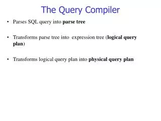
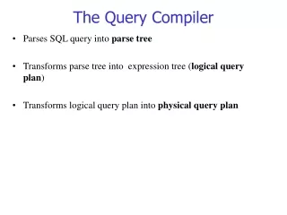
Database Systems II Query Compiler. Introduction. The Query Compiler translates an SQL query into a physical query plan, which can be executed, in three steps: The query is parsed and represented as a parse tree .

E N D
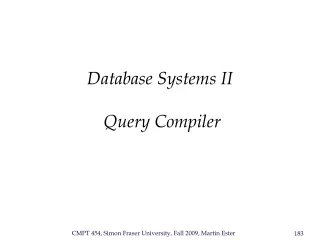
Introduction • The Query Compiler translates an SQL query into a physical query plan, which can be executed, in three steps: • The query is parsed and represented as a parse tree. • The parse tree is converted into a relational algebra expression tree (logical query plan). • The logical query plan is refined into a physical query plan, which also specifies the algorithms used in each step and the way in which data is obtained.
Introduction SQL query parse parse tree convert answer logical query plan execute query rewrite Pi “improved” l.q.p pick best estimate result sizes {(P1,C1),(P2,C2)...} l.q.p. +sizes estimate costs consider physical plans {P1,P2,…..}
Introduction Example • SELECT B,D • FROM R,S • WHERE R.A = “c” S.E = 2 R.C=S.C • Conceptual evaluation strategy: • Perform cartesian product, • Apply selection, and • Project to specified attributes. • Use as starting point for optimization.
Example B,D sR.A=“c” S.E=2 R.C=S.C X R S Introduction B,D [sR.A=“c” S.E=2 R.C = S.C (RXS)]
Introduction Example B,D sR.A = “c”sS.E = 2 R S natural join This logical query plan is equivalent. It is more efficient, since it reduces the sizes of the intermediate tables.
Introduction Example Needs to be refined into physical query plan. E.g., use R.A and S.C indexes as follows: (1) Use R.A index to select R tuples with R.A = “c” (2) For each R.C value found, use S.C index to find matching tuples (3) Eliminate S tuples S.E 2 (4) Join matching R,S tuples, project B,D attributes and place in result
Parsing Parse Trees Nodes correspond to either atoms (terminal symbols) or syntactic categories (non-terminal symbols). An atom is a lexical element such as a keyord, name of an attribute or relation, constant, operator, parenthesis. A syntactic category denotes a family of query subparts that all play the same role within a query, e.g. Condition. Syntactic categories are enclosed in triangular brackets, e.g. <Condition>.
Parsing Example SELECT title FROM StarsIn WHERE starName IN (SELECT name FROM MovieStar WHERE birthdate LIKE ‘%1960’);
Parsing <Query> <SFW> SELECT <SelList> FROM <FromList> WHERE <Condition> <Attribute> <RelName> <Tuple> IN <Query> title StarsIn <Attribute> ( <Query> ) starName <SFW> SELECT <SelList> FROM <FromList> WHERE <Condition> <Attribute> <RelName> <Attribute> LIKE <Pattern> name MovieStar birthDate ‘%1960’
Parsing Grammar for SQL The following grammar describes a simple subset of SQL. Queries <Query>::= SELECT <SelList> FROM <FromList> WHERE <Condition> ; Selection lists <SelList>::= <Attribute>, <SelList> <SelList>::= <Attribute> From lists <FromList>::= <Relation>, <FromList> <FromList>::= <Relation>
Parsing Grammar for SQL • Conditions <Condition>::= <Condition> AND <Condition><Condition>::= <Attribute> IN (<Query>)<Condition>::= <Attribute> = <Attribute> <Condition>::= <Attribute> LIKE <Pattern> • Syntactic categories Relation and Attribute are not defined by grammar rules, but by the database schema. • Syntactic category Pattern defined as some regular expression.
Conversion to Query Plan • How to convert a parse tree into a logical query plan, i.e. a relational algebra expression? • Queries with conditions without subqueries are easy: • Form Cartesian product of all relations in <FromList>. • Apply a selection sc where C is given by <Condition>. • Finally apply a projection pL where L is the list of attributes in <SelList>. • Queries involving subqueries are more difficult. • Remove subqueries from conditions and represent them by a two-argument selection in the logical query plan. • See the textbook for details.
Algebraic Laws for Query Plans Introduction Algebraic laws allow us to transform a Relational Algebra (RA) expression into an equivalent one. Two RA expressions are equivalent if, for all database instances, they produce the same answer. The resulting expression may have a more efficient physical query plan. Algebraic laws are used in the query rewrite phase.
Algebraic Laws for Query Plans Introduction Commutative law: Order of arguments does not matter. x + y = y + x Associative law: May group two uses of the operator either from the left or the right. (x + y) + z = x + (y + z) Operators that are commutative and associative can be grouped and ordered arbitrarily.
Algebraic Laws for Query Plans Natural Join, Cartesian Product and Union R S = S R (R S) T = R (S T) R x S = S x R (R x S) x T = R x (S x T) R U S = S U R R U (S U T) = (R U S) U T
Algebraic Laws for Query Plans Natural Join, Cartesian Product and Union R S = S R To prove this law, need to show that any tuple resulting from the left side expression is also produced by the right side expression, and vice versa. Suppose tuple t is in R S. There must be tuples r in R and s in S that agree with t on all shared attributes. If we evaluate S R, tuples s and r will againresult in t.
Algebraic Laws for Query Plans Natural Join, Cartesian Product and Union R S = S R Note that the order of attributes within a tuple doesnot matter (carry attribute names along). Relation as bag of tuplesAccording to the same reasoning, the number of copies of t must be identical on both sides. The other direction of the proof is essentially the same, given the symmetry of S and R.
Algebraic Laws for Query Plans Selection sp1p2(R) = sp1vp2(R) = sp1 [ sp2 (R)] [ sp1 (R)] U [ sp2 (R)] sp1 [ sp2 (R)] = sp2 [ sp1 (R)] Simple conditions p1 or p2 may be pushed down further than the complex condition.
Algebraic Laws for Query Plans Bag Union What about the union of relations with duplicates (bags)? R = {a,a,b,b,b,c} S = {b,b,c,c,d} R U S = ? Number of occurrences either SUM or MAX of occurrences in the imput relations. SUM: R U S = {a,a,b,b,b,b,b,c,c,c,d} MAX: R U S = {a,a,b,b,b,c,c,d}
Algebraic Laws for Query Plans Selection s p1vp2 (R) = sp1(R) U sp2(R) MAX implementation of union makes rule work. R={a,a,b,b,b,c} p1 satisfied by a,b, p2 satisfied by b,c sp1vp2 (R) = {a,a,b,b,b,c}sp1(R) = {a,a,b,b,b}sp2(R) = {b,b,b,c}sp1(R) U sp2 (R) = {a,a,b,b,b,c}
Algebraic Laws for Query Plans Selection s p1vp2 (R) = sp1(R) U sp2(R) SUM implementation of union makes more sense. Senators (……) Reps (……) T1 = p yr,state Senators, T2 = pyr,state Reps T1 Yr State T2 Yr State 97 CA 99 CA 99 CA 99 CA 98 AZ 98 CA Use SUM implementation, but then some laws do not hold. Union?
Algebraic Laws for Query Plans Selection and Set Operations sp(R U S) = sp(R) U sp(S) sp(R - S) = sp(R) - S = sp(R) - sp(S)
Algebraic Laws for Query Plans Selection and Join p: predicate with only R attributes q: predicate with only S attributes m: predicate with attributes from R and S sp (R S) = sq (R S) = [sp (R)] S R [sq (S)]
Algebraic Laws for Query Plans Selection and Join spq (R S) = [sp (R)] [sq (S)] spqm (R S) = sm[(sp R) (sq S)] spvq (R S) = [(sp R) S] U [R(sq S)]
Algebraic Laws for Query Plans Selection and Join spq (R S) = sp [sq (R S) ] = sp[ R sq (S) ] = [sp (R)] [sq (S)]
Algebraic Laws for Query Plans Projection X: set of attributes Y: set of attributes XY: X U Y pxy (R) = May introduce projection anywhere in an expression tree as long as it eliminates no attributes needed by an operator above and no attributes that are in result px [py (R)]
pxz px Algebraic Laws for Query Plans Projection and Selection X: subset of R attributes Z: attributes in predicate P (subset of R attributes) px (spR) = Need to keep attributes for the selection and for the result {sp [ px (R) ]}
Algebraic Laws for Query Plans Projection, Selection and Join pxy {sp(R S)} = pxy {sp[pxz (R) pyz’ (S)]} Y: subset of S attributes z = subset of R attributes used in P z’ = subset of S attributes used in P
Improving Logical Query Plans Introduction How to apply the algebraic laws to improve a logical query plan? Goal: minimize the size (number of tuples, number of attributes) of intermediate results. Push selections down in the expression tree as far as possible. Push down projections, or add new projections where applicable.
Improving Logical Query Plans Pushing Selections Replace the left side of one of these (and similar) rules by the right side: Can greatly reduce the number of tuples of intermediate results. sp1p2 (R) sp1 [sp2 (R)] sp (R S) [sp (R)] S
Improving Logical Query Plans Pushing Projections Replace the left side of one of this (and similar) rules by the right side: Reduces the number of attributes of intermediate results and possibly also the number of tuples. px [sp (R)] px {sp [pxz (R)]}
Improving Logical Query Plans Pushing Projections Consider the following example: R(A,B,C,D,E) P: (A=3) (B=“cat”) Compare pE {sp (R)} vs. pE {sp{pABE(R)}}
Improving Logical Query Plans Pushing Projections What if we have indexes on A and B? B = “cat” A=3 Intersect pointers to get pointers to matching tuples Efficiency of logical query plan may depend on choices made during refinement to physical plan. No transformation is always good!
Improving Logical Query Plans Grouping Associative / Commutative Operators For operators which are commutative and associative, we can order and group their arguments arbitrarily. In particular: natural join, union, intersection. As the last step to produce the final logical query plan, group nodes with the same (associative and commutative) operator into one n-ary node. Best grouping and ordering determined during the generation of physical query plan.
Improving Logical Query Plans Grouping Associative / Commutative Operators U C D E U C D E A B A B
From Logical to Physical Plans • So far, we have parsed and transformed an SQL query into an optimized logical query plan. • In order to refine the logical query plan into a physical query plan, we • consider alternative physical plans, • estimate their cost, and • pick the plan with the least (estimated) cost. • We have to estimate the cost of a plan without executing it. And we have to do that efficiently!
From Logical to Physical Plans • When creating a physical query plan, we have to decide on the following issues. • order and grouping of operations that are associative and commutative, • algorithm for each operator in the logical plan, • additional operators which are not represented in the logical plan, e.g. sorting, • the way in which intermediate results are passed from one operator to the next, e.g. by storing on disk or passing one tuple at a time.
Estimating the Cost of Operations Intermediate relations are the output of some relational operator and the input of another one. The size of intermediate relations has a major impact on the cost of a physical query plan. It impacts in particular - the choice of an implementation for the various operators and - the grouping and order of commutative / associative operators.
Estimating the Cost of Operations • A method for estimating the size of an intermediate relation should be • reasonably accurate,- efficiently computable,- not depend on how that relation is computed. • We want to rank alternative query plans w.r.t. their estimated costs. • Accuracy of the absolute values of the estimates not as important as the accuracy of their ranks.
Estimating the Cost of Operations • Size estimates make use of the followingstatistics for relation R: • T(R) : # tuples in R • S(R) : # of bytes in each R tuple • B(R): # of blocks to hold all R tuples • V(R, A) : # distinct values for attribute Ain R. • MIN(R,A): minimum value of attribute A in R. • MAX(R,A): maximum value of attribute A in R.HIST(R,A): histogram for attribute A in R. • Statistics need to be maintained up-to-dateunder database modifications!
A B C D cat 1 10 a cat 1 20 b dog 1 30 a dog 1 40 c bat 1 50 d Estimating the Cost of Operations R A: 20 byte string B: 4 byte integer C: 8 byte date D: 5 byte string T(R) = 5 S(R) = 37 V(R,A) = 3 V(R,C) = 5 V(R,B) = 1 V(R,D) = 4
Estimating the Cost of Operations • Size estimate for W = R1 x R2 • T(W) = T(R1) T(R2) • S(W) = S(R1) + S(R2) • Size estimate for W = sA=a (R) • Assumption: values of A are uniformly distributed over the attribute domain • T(W) = T(R)/V(R,A)S(W) = S(R)
Estimating the Cost of Operations • Size estimate for W = sz val (R) • Solution 1: on average, half of the tuples will satisfy an inequality condition • T(W) = T(R)/2 • Solution 2: more selective queries are more frequent, e.g. professors who earn more than $200’000 (rather than less than $200’000) • T(W) = T(R)/3
Estimating the Cost of Operations Solution 3: estimate the number of attributevalues in query range Use minimum and maximum value to define range of the attribute domain. Assume uniform distribution of valuesover the attribute domain. Estimate is the fraction of the domain thatfalls into the query range.
Estimating the Cost of Operations R Z MIN(R,Z)=1 V(R,Z)=10 W= sz 15 (R) MAX(R,Z)=20 f = 20-15+1 = 6 (fraction of range) 20-1+1 20 T(W) = f T(R)
Estimating the Cost of Operations Size estimate for W = R1 R2 Consider only natural join of R1(X,Y) and R2(Y,Z). We do not know how the Y values in R1 and R2 relate:- disjoint, i.e. T(R1 R2) = 0,- Y may be a foreign key of R1 and the primary key of R2, i.e. T(R1 R2) = T(R1),- all the R1 and all the R2 tuples have the same Y value, i.e. T(R1 R2) = T(R1) T(R2).
Estimating the Cost of Operations Make several simplifying assumptions. Containment of value sets: V(R1,Y) V(R2,Y) every Y value in R1 is in R2 V(R2,Y) V(R1,Y) every Y value in R2 is in R1 This assumption is satisfied when Y is foreign key in R1 and primary key in R2. Is also approximately true in many other cases.
Estimating the Cost of Operations Preservation of value sets:If A is an attribute of R1 but not of R2, thenV(R1 R2,A) = V(R1,A). Again, holds if the join attribute Y is foreign key in R1 and primary key in R2. Can only be violated if there are “dangling tuples” in R1, i.e. R1 tuples that have no matching partner in R2.
Estimating the Cost of Operations Uniform distribution of attribute values: the values of attribute A are uniformly distributed over their domain, i.e. P(A=a1) =P(A=a2) = . . . = P(A=ak). This assumption is necessary to make cost estimation tractable. It is often violated, but nevertheless allows reasonably accurate ranking of query plans.