CS433 Modeling and Simulation Lecture 11 Continuous Markov Chains

1. Al-Imam Mohammad Ibn Saud University CS433Modeling and SimulationLecture 11 Continuous Markov Chains Dr. Anis Koubâa 01 May 2009

2. Goals for Today • Understand the Markov property in the Continuous Case • Understand the difference between continuous time and discrete time Markov Chains • Learn how to use Continuous Markov Chains for modelling stochastic processes

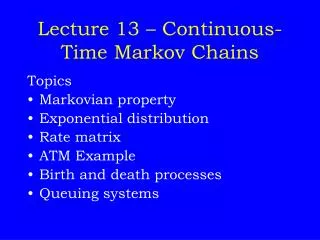
3. “Discrete Time” versus “Continuous Time” Fixed Time Discrete Time t=1 t=1 time 4 3 1 2 0 Events occur at known points in time Continuous Time Variable Time t2=v-u t3=t-v t1=u-s time v t u s Events occur at any point in time

4. Definition (WiKi): Continuous-Time Markov Chains • In probability theory, a Continuous-Time Markov Process (CTMC) is a stochastic process{ X(t) : t ≥ 0 } that satisfies the Markov property and takes values from a set called the state space. • The Markov property states that at any times s > t > 0, the conditional probability distribution of the process at time s given the whole history of the process up to and including time t, depends only on the state of the process at time t. • In effect, the state of the process at time s is conditionally independent of the history of the process before time t, given the state of the process at time t.

5. Definition 1: Continuous-Time Markov Chains • A stochastic process {X(t), t 0} is a Continuous-Time Markov Chain (CTMC) if for all 0  s  t and non-negative integers i, j, x(u), such that 0  u < s, • In addition, if this probability is independent from s and t, then the CTMC has stationary transition probabilities: X(t)=j X(u)=x(u) X(s)=i t t u s مدة زمنية الماضي المستقبل الحاضر

6. Differences between Continuous-Time and Discrete-Time Markov Chains time 4 3 1 2 0 Events occur at known points in time Fixed Time Continuous Time Discrete Time Variable Time t=1 t=1 t2=v-u t3=t-v t1=u-s time u s v t Events occur at any point in time

7. Definition 2: Continuous-Time Markov Chains • A stochastic process {X(t), t 0} is a Continuous-Time Markov Chain (CTMC) if • The amount of time spent in state i before making a transition to a different state is exponentially distributedwith rate a parameter vi, • When the process leaves state i, it enters state j with a probability pij, where pii = 0 and • All transitions and times are independent (in particular, the transition probability out of a state is independent of the time spent in the state). Summary: The CTMC process moves from state to state according to DTMC, and the time spent in each state is exponentially distributed

8. Differences between DISCRETE and CONTINOUS DTMC process CTMC process Summary: The CTMC process moves from state to state according to DTMC, and the time spent in each state is exponentially distributed

9. Five Minutes Break You are free to discuss with your classmates about the previous slides, or to refresh a bit, or to ask questions.

10. Chapman Kolmogorov: Transition Function دالة الانتقال • Define the Transition Function (like Transition Probability in DTMC) • Using the Markov (memoryless) property

11. Time Homogeneous Case Transition Matrix State Holding Time Transition Rate Transition Probability

12. Homogeneous Case The transition rate matrix qij is the transition ratethat the chain enters state j from state i ni=-qii is the transition ratethat the chain leaves state i Discrete Markov Chain Continuous Markov Chain Pij qki=nk . Pki qji=nj . Pji j k i i j Pji qij=ni . Pij qik=ni . Pik Pij: Transition Probability, qij input rate from i to j, ni output rate Transition Time is random Pij: Transition Probability Transition Time is deterministic (each slot)

13. Continuous Markov Chain Continuous Markov Chain qik=ni . Pik qij=ni . Pij • Pij: Transition Probability, • qij input rate of state j from state i, • ni output rate from state i for • all other neighbor states • Transition Time is randoms qki=nk . Pki qji=nj . Pji Discrete Markov Chain Pij j k i i j Pji Pij: Transition Probability Transition Time is Known (each slot)

14. Transition ProbabilityMatrix in Homogeneous Case • Thus, if P(t) is the Transition Matrix AFTERa time period t • pij(0) is the instantaneous transition function from i to j

15. Next: State Holding Time Two Minutes Break You are free to discuss with your classmates about the previous slides, or to refresh a bit, or to ask questions.

16. State Holding and Transition Time • In a CTMC, the process makes a transition from one state to another, after it has spent an amount of time on the state it starts from. This amount of time is defined as the state holding time. • Theorem: State Holding Time of CTMC • The state holding time Ti:= inf {t: Xt≠ i| X0 = i} in a state i of a Continuous-Time Markov Chain • Satisfies the Memoryless Property • Is Exponentially Distributed with the parameter ni • Theorem: Transition Time in a CTMC • The time Tij:= inf {t: Xt= j | X0 = i}spent in a state i before a transition to state j is exponentially distributed with the parameter qij

17. State Holding Time: Proofs • Suppose our continuous time Markov Chain has just arrived in state i. Define the random variable Ti to be the length of time the process spends in state i before moving to a different state. We call Ti the holding time in state i. • The Markov Property implies • the distribution of how much longer you’ll be in a given • state i is independent of how long you’ve already been there. • Proof (1) (by contradiction): • Suppose it is time s, you are in state i, and • i.e., the amount of time you have already been in state i is relevant in • predicting how much longer you will be there. Then for any time r < s, • whether or not you were in state i at time r is relevant in predicting • whether you will be in state i or a different state j at some future time • s + t. Thus • which violates the Markov Property. • Proof (2): • The only distribution satisfying the memoryless property is the exponential distribution. Thus, the result in (2).

18. Example: Computer System Assume a computer system where jobs arrive according to a Poisson process with rate λ. Each job is processed using a First In First Out (FIFO) policy. The processing time of each job is exponential with rate μ. The computer has a buffer to store up to two jobs that wait for processing. Jobs that find the buffer full are lost.

19. Example: Computer System Questions Draw the state transition diagram. Find the Rate Transition Matrix Q. Find the State Transition Matrix P

20. Example a a a 0 1 2 3 a d d d • The rate transition matrix is given by • The state transition matrix is given by

21. Transient State Probabilities

22. State Probabilities and Transient Analysis • Similar to the discrete-time case, we define • In vector form • With initial probabilities • Using our previous notation (for homogeneous MC) Obtaining a general solution is not easy!

23. Steady State Probabilities

24. Steady State Analysis • Often we are interested in the “long-run” probabilistic behavior of the Markov chain, i.e., • These are referred to as steady state probabilitiesor equilibrium state probabilities or stationary state probabilities • As with the discrete-time case, we need to address the following questions • Under what conditions do the limits exist? • If they exist, do they form legitimate probabilities? • How can we evaluate these limits?

25. Steady State Analysis • Theorem: In an irreducible continuous-time Markov Chain consisting of positive recurrent states, a unique stationary state probability vector π with • These vectors are independent of the initial state probability and can be obtained by solving

26. Example a a a 0 1 2 3 a d d d • For the previous example, with the above transition function, what are the steady state probabilities • Solve

27. Example • The solution is obtained

28. Uniformization of Makov Chains

29. Uniformization of Markov Chains • In general, discrete-time models are easier to work with, and computers (that are needed to solve such models) operate in discrete-time • Thus, we need a way to turn continuous-time to discrete-time Markov Chains • Uniformization Procedure • Recall that the total rate out of statei is –qii=n(i). • Pick a uniform rateγsuch that γ≥ n (i)for all states i. • The difference γ-n (i)implies a “fictitious” event that returns the MC back to state i (self loop).

30. Uniformization of Markov Chains j j … qij … i k Uniformization i k qik … … • Uniformization Procedure • Let PUijbe the transition probability from state I to state j for the discrete-time uniformized Markov Chain, then

31. End of Chapter