Download
1 / 39
650 likes | 1.44k Views
Darcy’s law. Groundwater Hydraulics Daene C. McKinney. Outline. Darcy’s Law Hydraulic Conductivity Heterogeneity and Anisotropy Refraction of Streamlines Generalized Darcy’s Law. Darcy. http:// biosystems.okstate.edu /Darcy/English/ index.htm. Darcy’s Experiments. Discharge is

E N D
Darcy’s law Groundwater Hydraulics Daene C. McKinney
Outline • Darcy’s Law • Hydraulic Conductivity • Heterogeneity and Anisotropy • Refraction of Streamlines • Generalized Darcy’s Law
Darcy http://biosystems.okstate.edu/Darcy/English/index.htm
Darcy’s Experiments • Discharge is Proportional to • Area • Head difference Inversely proportional to • Length • Coefficient of proportionality is K= hydraulic conductivity
Hydraulic Conductivity • Has dimensions of velocity [L/T] • A combined property of the medium and the fluid • Ease with which fluid moves through the medium k = cd2 intrinsic permeability ρ = density µ = dynamic viscosity g = specific weight Porous medium property Fluid properties
Groundwater Velocity • q - Specific discharge Discharge from a unit cross-section area of aquifer formation normal to the direction of flow. • v - Average velocity Average velocity of fluid flowing per unit cross-sectional area where flow is ONLY in pores.
Example h1 = 12m h2 = 12m • K= 1x10⁻⁵ m/s • f = 0.3 • Find q, Q, and v /” Flow Porous medium 10m 5 m L = 100m dh= (h2 - h1) = (10 m – 12 m) = -2 m J= dh/dx = (-2 m)/100 m = -0.02 m/m q= -KJ = -(1x10⁻⁵ m/s) x (-0.02 m/m) = 2x10⁻⁷ m/s Q= qA = (2x10⁻⁷ m/s) x 50 m2= 1x10⁻⁵ m3/s v = q/f= 2x10⁻⁷ m/s / 0.3 = 6.6x10⁻⁷m/s
Hydraulic Gradient Gradient vector points in the direction of greatest rate of increase of h Specific discharge vector points in the opposite direction of h
Well Pumping in an Aquifer Hydraulic gradient y Circular hydraulic head contours Dh K, conductivity, Is constant q Specific discharge x Well, Q h1 h2 h3 h1 < h2 < h3 Aquifer (plan view)
Validity of Darcy’s Law • We ignored kinetic energy (low velocity) • We assumed laminar flow • We can calculate a Reynolds Number for the flow q = Specific discharge d10 = effective grain size diameter • Darcy’s Law is valid for NR < 1 (maybe up to 10)
Specific Discharge vs Head Gradient Experiment shows this Re = 10 Re = 1 Darcy Law predicts this a q tan-1(a)= (1/K)
Estimating ConductivityKozeny – Carman Equation • Kozeny used bundle of capillary tubes model to derive an expression for permeability in terms of a constant (c) and the grain size (d) • So how do we get the parameters we need for this equation? Kozeny – Carman eq.
Measuring ConductivityPermeameter Lab Measurements • Darcy’s Law is useless unless we can measure the parameters • Set up a flow pattern such that • We can derive a solution • We can produce the flow pattern experimentally • Hydraulic Conductivity is measured in the lab with a permeameter • Steady or unsteady 1-D flow • Small cylindrical sample of medium
Measuring ConductivityConstant Head Permeameter • Flow is steady • Sample: Right circular cylinder • Length, L • Area, A • Constant head difference (h) is applied across the sample producing a flow rate Q • Darcy’s Law Continuous Flow head difference Overflow flow Outflow Q A Sample
Measuring ConductivityFalling Head Permeameter • Flow rate in the tube must equal that in the column Initial head Final head flow Outflow Q Sample
Heterogeneity and Anisotropy • Homogeneous • Properties same at every point • Heterogeneous • Properties different at every point • Isotropic • Properties same in every direction • Anisotropic • Properties different in different directions • Often results from stratification during sedimentation www.usgs.gov
Example • a= ???, b= 4.673x10⁻¹⁰ m2/N, g= 9798 N/m3, • S = 6.8x10⁻⁴, b = 50 m, f= 0.25, • Saquifer= gabb= ??? • Swater= gbfb • % storage attributable to water expansion • %storage attributable to aquifer expansion
Layered Porous Media(Flow Parallel to Layers) Piezometric surface Dh h1 h2 datum Q b W
Layered Porous Media(Flow Perpendicular to Layers) Piezometric surface Dh1 Dh2 Dh Dh3 Q b Q L1 L2 L3 L
Example • Find average K Flow Q
Example Flow Q • Find average K
Anisotrpoic Porous Media • General relationship between specific discharge and hydraulic gradient
Principal Directions • Often we can align the coordinate axes in the principal directions of layering • Horizontal conductivity often order of magnitude larger than vertical conductivity
Flow between 2 adjacent flow lines For the squares of the flow net so For entire flow net, total head loss h is divided into n squares If flow is divided into m channels by flow lines
Flow lines are perpendicular to water table contours Flow lines are parallel to impermeable boundaries KU/KL = 1/50 KU/KL = 50
Contour Map of Groundwater Levels • Contours of groundwater level (equipotential lines) and Flowlines (perpendicular to equipotiential lines) indicate areas of recharge and discharge
Groundwater Flow Direction • Water level measurements from three wells can be used to determine groundwater flow direction Groundwater Contours hi > hj > hk hi Head Gradient, J hj hk h1(x1,y1) h3(x3,y3) z y Groundwater Flow, Q h2(x2,y2) x
Groundwater Flow Direction Head gradient = Magnitude of head gradient = Angle of head gradient =
Groundwater Flow Direction Head Gradient, J h1(x1,y1) h3(x3,y3) z Equation of a plane in 2D y Groundwater Flow, Q 3 points can be used to define a plane h2(x2,y2) x Set of linear equations can be solved for a, b and c given (xi, hi, i=1, 2, 3)
Groundwater Flow Direction Negative of head gradient in x direction Negative of head gradient in y direction Magnitude of head gradient Direction of flow
Example Find: y Well 2 (200 m, 340 m) 55.11 m Magnitude of head gradient Direction of flow Well 1 (0 m,0 m) 57.79 m x Well 3 (190 m, -150 m) 52.80 m
Example Well 2 (200, 340) 55.11 m x q = -5.3 deg Well 1 (0,0) 57.79 m Well 3 (190, -150) 52.80 m
Refraction of Streamlines • Vertical component of velocity must be the same on both sides of interface • Head continuity along interface • So y Upper Formation x Lower Formation
Consider a leaky confined aquifer with 4.5 m/d horizontal hydraulic conductivity is overlain by an aquitard with 0.052 m/d vertical hydraulic conductivity. If the flow in the aquitard is in the downward direction and makes an angle of 5o with the vertical, determine q2.
Summary • Properties – Aquifer Storage • Darcy’s Law • Darcy’s Experiment • Specific Discharge • Average Velocity • Validity of Darcy’s Law • Hydraulic Conductivity • Permeability • Kozeny-Carman Equation • Constant Head Permeameter • Falling Head Permeameter • Heterogeneity and Anisotropy • Layered Porous Media • Refraction of Streamlines • Generalized Darcy’s Law
Example Flow Q
Example Flow Q