Download
1 / 32
320 likes | 773 Views
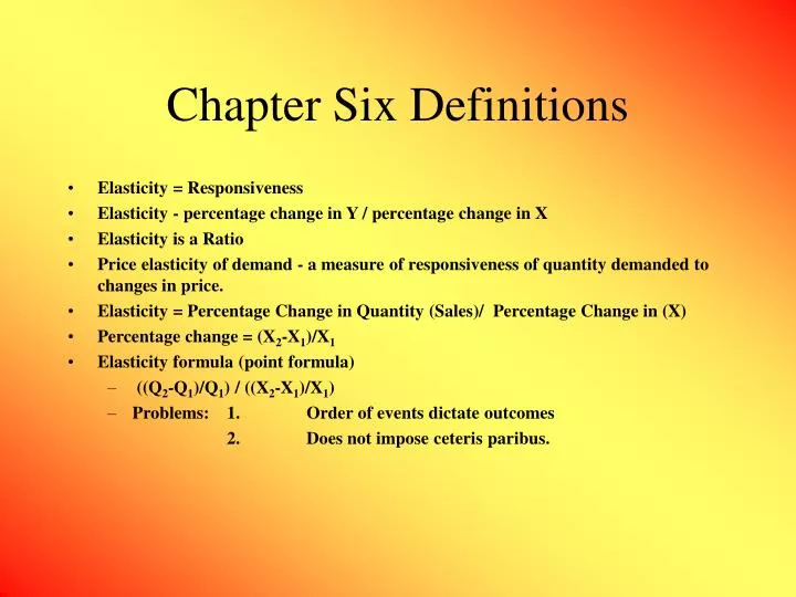
Chapter Six Definitions. Elasticity = Responsiveness Elasticity - percentage change in Y / percentage change in X Elasticity is a Ratio Price elasticity of demand - a measure of responsiveness of quantity demanded to changes in price.

E N D
Chapter Six Definitions • Elasticity = Responsiveness • Elasticity - percentage change in Y / percentage change in X • Elasticity is a Ratio • Price elasticity of demand - a measure of responsiveness of quantity demanded to changes in price. • Elasticity = Percentage Change in Quantity (Sales)/ Percentage Change in (X) • Percentage change = (X2-X1)/X1 • Elasticity formula (point formula) • ((Q2-Q1)/Q1) / ((X2-X1)/X1) • Problems: 1. Order of events dictate outcomes 2. Does not impose ceteris paribus.
Chapter Six, Cont. • Elasticity formula (arc formula) ((Q2-Q1)/((Q2+Q1)/2)) / ((X2-X1)/((X2+X1)/2)) Problems: 1. Does not impose ceteris paribus • Elasticity formula (slope formula) • Elasticity = %ΔQ / %ΔP = ((Q2-Q1)/Q1) / ((P2-P1)/P1) • Note: Q2-Q1 = ΔQ and P2-P1 = ΔP • Therefore: Elasticity = ΔQ /Q / ΔP/P • Note: If you divide by a fraction you multiply by the reciprocal • Therefore: Elasticity = ΔQ /Q * P/ΔP • or Elasticity = ΔQ / ΔP * P/Q • Where do we get ΔQ / ΔP? • This is the inverse slope of the demand curve, which we can estimate empirically imposing ceteris paribus.
Chapter Six, cont. • Interpretation of Price Elasticity • % change in Q > % change in P (elastic or responsive) Ep < -1 • % change in Q < % change in P (inelastic or unresponsive) Ep > -1 • % change in Q = % change in P (unitary elastic) Ep = -1 • Total Revenue = Price * Quantity = Total dollar value of units sold • If % change in Q > % change in P decreasing the price will increase TR • If % change in Q < % change in P increasing the price will increase TR • Profit = Total Revenue - Total Cost • If demand is inelastic (i.e. % change in Q < % change in P) an increase in price will increase TR. • Because Q falls (law of demand), so too will Total Cost • Why? Total Cost (which we will discuss later) is an increasing function of output. The more you produce, the higher your total cost. • Consequently, if demand is inelastic, a firm can raise its price and increase its profits.
Chapter Six, Cont. • Determinants of price elasticity of demand: Substitutes and Elasticity • a. Time • b. Necessity vs. Luxury • c. More specific the good the more elastic demand • d. Price of the good relative to income • Cross price elasticity of demand = % change in quantity / % change in the price of another good • Income elasticity = % change in quantity / % change in income
Summarizing Demand • The Law of Demand - Quantity demanded rises as price falls, ceteris paribus. Quantity demanded falls as price rises, ceteris paribus • The Law of Demand is based upon Gossen’s First and Second Laws. • The Law of Demand gives us the Demand Curve • Via own-price elasticity, we move from the demand curve to total revenue. • Total Revenue = Price * Quantity • Without own-price elasticity we do not know how changes in price and quantity will impact total revenue. • The variation in total revenue gives us the concept of marginal revenue. • Marginal Revenue - amount of revenue from the last unit sold. • the rate of change in total revenue • the slope of the total revenue curve. • If demand is downward sloping, then price will exceed marginal revenue. In other words, the amount of revenue generated by an additional sale will be less than the price the firm charges. • Why? To increase quantity the firm will need to lower the price, not just for the last unit sold, but also for every unit the firm wishes to sell.
Profit, Total Revenue, Total Cost • Profit = Total Revenue - Total Cost • Accounting Profit = Total Revenue - Explicit Costs • Economic Profit = Total Revenue - (explicit and implicit cost) • Normal Profit - A level of profit that is just sufficient to maintain ownership. • Total Cost = Explicit + Implicit Costs • Total Cost - explicit payments to the factors of production plus the opportunity cost of the factors provided by the owner of the firm. • Remember, total cost includes the owner’s wage, or a normal rate of return to the owner.
The Firm Basics • Production - the transformation of factors into goods and services. • Firm - an economic institution that transforms factors of production into goods and services. • Shirking - the behavior of a worker who is putting forth less than the agreed to effort. • Residual claimant - persons who share in the profits of the firm • Why would firms pay efficiency wages? a. The Gift exchange hypothesis b. Worker turnover c. Worker quality
The Short-Run • Long-run - a firm chooses among all possible production techniques • Short-run - the firm is constrained in regard to what production decisions it can make. • Short run - the longest period of time during which at least one of the inputs used in a production process cannot be varied. • Law of Diminishing Returns - As the amount of a variable input is increased, holding all else constant, the rate of increase in output will eventually decline. • Law of Diminishing Marginal Productivity - as more and more of a variable input is added to an existing fixed input, eventually the additional output one gets from that individual input is going to fall. • The Law of Diminishing Returns is the foundation on which we build our discussion of Total Cost.
Marginal Product and Average Product • Marginal product - the additional output that will be forthcoming from an additional worker, other inputs constant. • The change in total product that occurs in response to a unit change in a variable input (ceteris paribus). • The amount of output produced by the last unit of the input hired. • Change in total product / Change in an input • Slope of the total product curve • Rate of change in total product • Average Productivity - output per worker. • Total product / Inputs hired
Introduction to Labor Economics • Value Marginal Product = Marginal Product of Labor * Price of Output • Relevant when the firm has no control over market price. • Marginal Revenue Product = Marginal Product of Labor * Marginal Revenue of Output • Relevant when the firm has some control over market price. • Hume’s Dictum: “That what ought to be cannot be derived from what is” • Joan Robinson (1933) “What is actually meant by exploitation is usually that the wage is less than the marginal revenue product.” • The Gerald Scully approach • i. Estimate the value of a win. • Revenue = f(wins, ...) • ii. Estimate the value of the player’s actions in terms of wins. • Wins = f(player and team statistics) • iii. Compare a player’s estimated MRP to the player’s wage. • The Anthony Krautman approach • If the market is competitive..... Salary = MRP • Salary = f(player statistics) • From this we can learn the value of a player’s statistics and thus analyze the value of non-free agents.
Short-Run Costs • Fixed input - an input whose quantity cannot be changed as output changes in the short run. • Variable input - an input whose quantity can be changed as output changes in the short-run. • Total Costs = Fixed Costs + Variable Costs • Fixed costs - costs that are spent and cannot be changed in the period of time under consideration. • costs of production that do not change as output changes (i.e. land and capital) • Variable costs - costs of production that change as output changes (i.e. labor and raw materials) • Marginal Cost - the increase in total cost associated with a one-unit increase in production. • Change in total cost / Change in output • Slope of the total cost curve • Rate of change in total cost • Average Total Cost = Total cost / quantity that is produced • Average Total Cost = Average Fixed Cost + Average Variable Cost • Minimum Average Total Cost represents the cheapest (in terms of per-unit costs) point of production. • When ATC is minimized - ATC = MC
Summarizing Total Cost • TC = FC + VC • ATC = TC/Q • ATC = AFC + AVC • MC = change in TC/change in q • Production, Total Cost and Marginal Cost • The Law of Diminishing Returns tells us that as labor increases, output will increase eventually at a diminishing rate. • If additional labor is less productive, than total cost will be increasing at an increasing rate. • Hence, marginal cost, after diminishing returns has set in, increases as output increases.
Profit Maximization vs. Average Cost Minimization • The profit maximizing rule >>>>> MR = MC Why? • If MR > MC profit will rise • If MR < MC profit will decline • When MR = MC then profit will be maximized. • What is the elasticity of demand when profit is maximized? • Average cost is minimized when ATC = MC. • What is the significance of the average cost minimizing level of output? This is the most efficient level of production in the short-run, but not necessarily profit maximization.
Long-Run Production and Cost • Long run - the shortest period of time required to alter the amounts of all inputs used in a production process. • A period of time long enough for all inputs to be varied. • Economies of scale - reductions in the minimum average cost that come about through increasing plant size. • Constant returns to scale - increases in plant size do not affect minimum average cost. • Diseconomies of scale - increases in plant size increase minimum average cost. • Long run average total cost is a summary of our best short-run cost possibilities. • Technical efficiency - as few inputs as possible are used to produce a given output. • Economic efficiency - the method that produces a given level of output at the lowest possible cost. • Economic efficiency is achieved when the amount of productivity received from each input per dollar spent is equal. • MP1/P1 = MP2/P2 = ....... = MPn/Pn
Industrial Organization • Industrial Organization: The study of the structure of firms and markets and of their interactions. • Market Structure - the particular environment of a firm, the characteristics of which influence the firm’s pricing and output decisions. • The continuum of market structures Perfect competition -------------------------------Monopoly • The study of perfect competition and monopoly provides the extremes, so we can see the limits of what is possible.
Perfect Competition 1. The number of firms is large. • Free entry and exit - there are no barriers to entry Barriers to entry - social, political, or economic impediments that prevent other firms from entering a market. 3. The product is homogenous (i.e. no product differentiation). • There is complete information: buyers and sellers know about prices, product quality, and seller location. No seller has an advantage over another firm. • Selling firms are profit maximizing firms. As a result: A perfectly competitive firm is a price taker. • Price taker - a seller does not have the ability to control the price of the product it sells; it takes the price determined in the market. • Market Power - ability to alter the market price of a good or service. • Competitive Firm - a firm without market power.
The Shut-Down Decision • Fixed costs must be paid whether or not the firm produces. • So the question facing the firm when considering whether to shutdown or not is – • Are the losses induced from production in excess of my fixed costs (losses induced from not producing)? • As long as some of the fixed costs are covered, production should continue. Proof of the Shut-Down Point • Profit = TR – TC Where TR = PQ TC = TVC + TFC • Profit = PQ - TVC - TFC • PQ > TVC then Profit will be greater than TFC • TVC = AVC*Q • PQ > AVC*Q then Profit will be greater than TFC • P > AVC then Profit will be greater than TFC • As long as price exceed average variable cost the firm should continue production, because profit exceed fixed costs.
The Conditions of Long-Run Competitive Equilibrium • In perfect competition P = MR • Therefore, if the firm is profit maximizing: P = MC • In the long-run, economic profit will be competed to zero. • Profit = TR – TC TR = PQ TC = ATC*Q Profit = PQ – ATC*Q Profit = [P – ATC]*Q If P = ATC then economic profit is zero. • If P = MC (because firms are profit maximizing) and P = ATC (because of competition) then P = MC = ATC. • What will the price equal in the long-run? The cost of production. • What does this mean? In the long-run, in perfect competition, firms will produce at maximum efficiency. • Resource allocative efficiency - the situation that exists when firms produce the quantity of output at which price equals marginal cost. • Productive efficiency - a situation that exists when a firm produces its output at the lowest possible per unit cost (lowest ATC).
Monopoly • Monopoly - a market structure in which one firm makes up the entire market. • Characteristics • 1. There is one seller • [as opposed to many small sellers] • 2. Product is unique • [as opposed to a homogenous good] • 3. Blockaded entry and exit • [as opposed to free entry and exit] • 4. Imperfect information • [as opposed to perfect information] • 5. Firm is a profit maximizer • As a result, the firm is a price maker • Price maker – firm can impact the price of the product it sells
Monopoly Myths • Myth one: Monopolies can charge whatever price they wish. • A monopoly is constrained by its level of demand. • Myth Two: A monopoly always makes an economic profit. • If demand is insufficient, P < ATC, and the firm will not make an economic profit. • If all monopolies made an economic profit, each small town would have the same assortment of goods and services offered in a larger city.
Monopoly vs. Perfect Competition • In perfect competition: P = MR = MC • In monopoly: P > MR P > MC MR = MC • So a monopoly does not produce the good according to the dictates of resource allocative efficiency. • In perfect competition in the long-run: P=MC=ATC • In monopoly: P may exceed ATC indefinitely • So a monopoly does not produce the good according to the dictates productive efficiency.
Social Costs of Monopoly • Deadweight Loss [Illustrate] • Rent-seeking - actions of individuals and groups who spend resources to influence public policy in the hope of redistributing income to themselves from others. • X-inefficiency • Price discrimination - to charge different prices to different individuals or groups of individuals
Barriers to Entry and Natural Monopoly • Legal barriers:Public franchises, patents, licenses Government created monopolies • Exclusive ownership or natural ability • Economies of scale • Natural Monopoly -An industry in which total market demand is met by a single firm while long run average total cost is still declining. • an industry in which a single firm can produce at a lower cost than can two or more firms.
Concentration Ratio • Are two firms in the same market? • F.M. Sherer: Rule of thumb - If cross price elasticity is 3 or greater the firms are in the same market. • Concentration ratio - the percentage of industry sales accounted by x number of firms in the industry. • Herfindahl index - an index of market concentration calculated by adding the squared value of individual market shares of all the firms in the industry. • < 1000 (unconcentrated) - Justice Department will act if merger raises the HHI by 100 points • > 1800 (concentrated - Justice Department will act if merger raises the HHI by 50 points. • Review Table 13-2
Limitations of Concentration Ratios • Global markets (impact of imports and exports) • National markets (proper geographic definition) • Industry definitions and product classes • Cross-price elasticity should assist in clearing up most confusion.
Monopolistic Competition • Monopolistic Competition - A market structure characterized by a large number of sellers of differentiated products. • Characteristics of Monopolistic Competition • Large number of buyers and sellers • Free entry and exit • Perfect information • Products are differentiated • Firms profit maximize • The differentiation of products results in a downward sloping demand curve. • Why? When price rises, demand does not go to zero. (i.e. brand loyalty)
Short-run vs. Long-run • Short-run: P>MC and potentially P>ATC • Long-run P>MC P=ATC • Key idea: MC does not equal ATC • Excess capacity theorem - in monopolistic competitor in long-run equilibrium will produce less output than the level of output that will minimize ATC. • Why? The product is differentiated. This means the demand curve is downward sloping. Hence, P > MR. • Question? Which is a better society: Monopolistic Competition or Perfect Competition • Edward Chamberlin - believed the difference between the cost of a perfect competitor and the cost of a monopolistic competitor was the cost of what he called “differentness” Chamberlin believed that if the differences were not important consumers would not pay. Is this necessarily true?
Oligopoly • Oligopoly - a market structure characterized by a few sellers and interdependent price/output decisions. • Characteristics • Few buyers and sellers (Heavily Concentrated) • Homogenous or Unique product • Barriers to entry • Imperfect information • Firms profit maximize • In Perfect Competition, Monopolistic Competition and Monopoly the decisions of one firm does not impact the decisions of other firms. There is no interdependence. This is not true in oligopoly, making it a very difficult market structure to examine. • Consequently, Oligopoly, unlike other market structures, is not best characterized by one model, but rather different models are used to discuss different aspects of these markets.
Oligopoly Models • The interdependence of firms prevents us from developing a universal oligopoly model • Models we will consider • Cartel • Kinked Demand Curve • Contestable Markets • Game Theory • Note: This is but a sample of the model we could consider.
Cartels, Kinked Demand, and Contestable Markets • Cartel - an organization of firms that reduces output and increases price in an effort to increase joint profits. • Primary problem with cartels: Firms always have an incentive to cheat. • The tendency to cheat can be illustrated. • The Kinked Demand Curve Model • Firms match price decreases, but do not match price increases. • This creates a kink in the demand curve. • Be able to explain why costs can change but profit maximizing output and price would the not in the kinked demand curve model. • Contestable Markets • There is free entry, and new firms can enter the market with the same cost as existing firms. • Exiting firms can easily dispose of their fixed assets, thus making exiting costless. • Conclusions of the model • 1. Number of firms does not indicate the competitive nature of the market. • 2. Economic profits can be small with few firms. • 3. Inefficient firms cannot exist in the industry • 4. If firms are encouraged to produce at the lowest possible cost P = ATC = MC
Game Theory • Game Theory - a mathematical technique used to analyze the behavior of decision makers. • the study of behavior in situations in which each party’s payoff directly depends on what another party does. • Characteristics of contestants. Decision makers • try to reach an optimal position through game playing or the use of strategic behavior. • are fully aware of the interactive process of the game. • anticipate the moves of other decision makers • Example: Two firms are determining how much to advertise. • The elements of the normal form game: • The players: Firm 1, Firm 2 • The strategies: High advertising, low advertising
Prisoner’s Dilemma • The payoffs: Are as follows (payoffs read 1,2) Firm 2 High Low High 40,40 100, 10 Firm 1 Low 10, 100 60,60 • Solving games • Equilibrium: no pressure for any participant to change his/hers action • Dominant strategy equilibrium: In this game, the dominant strategy for firm 1 and firm 2 is high. So the outcome of the game is 40,40. • This illustrates the prisoner’s dilemma: Games in which the equilibrium of the game is not the outcome the players would choose if they could perfectly cooperate. • REVIEW PAGE 300