Download
1 / 44
540 likes | 972 Views
Geographically weighted regression. Danlin Yu Yehua Dennis Wei Dept. of Geog., UWM. Outline of the presentation. Spatial non-stationarity: an example GWR – some definitions 6 good reasons using GWR Calibration and tests of GWR An example: housing hedonic model in Milwaukee

E N D
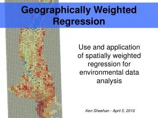
Geographically weighted regression Danlin Yu Yehua Dennis Wei Dept. of Geog., UWM
Outline of the presentation • Spatial non-stationarity: an example • GWR – some definitions • 6 good reasons using GWR • Calibration and tests of GWR • An example: housing hedonic model in Milwaukee • Further information
1. Stationary v.s non-stationary yi= i0 + i1x1i yi= 0 + 1x1i e1 e1 e2 e2 Stationary process Non-stationary process e4 e3 e3 e4 Assumed More realistic
Simpson’s paradox Spatially aggregated data Spatially disaggregated data House Price House density House density
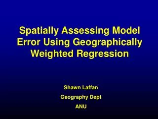
Stationary v.s. non-stationary • If non-stationarity is modeled by stationary models • Possible wrong conclusions might be drawn • Residuals of the model might be highly spatial autocorrelated
Why do relationships vary spatially? • Sampling variation • Nuisance variation, not real spatial non-stationarity • Relationships intrinsically different across space • Real spatial non-stationarity • Model misspecification • Can significant local variations be removed?
2. Some definitions • Spatial non-stationarity: the same stimulus provokes a different response in different parts of the study region • Global models: statements about processes which are assumed to be stationary and as such are location independent
Some definitions • Local models: spatial decompositions of global models, the results of local models are location dependent – a characteristic we usually anticipate from geographic (spatial) data
Regression • Regression establishes relationship among a dependent variable and a set of independent variable(s) • A typical linear regression model looks like: • yi=0 + 1x1i+ 2x2i+……+ nxni+i • With yithe dependent variable, xji (j from 1 to n) the set of independent variables, and ithe residual, all at location i
Regression • When applied to spatial data, as can be seen, it assumes a stationary spatial process • The same stimulus provokes the same response in all parts of the study region • Highly untenable for spatial process
Geographically weighted regression • Local statistical technique to analyze spatial variations in relationships • Spatial non-stationarity is assumed and will be tested • Based on the “First Law of Geography”: everything is related with everything else, but closer things are more related
GWR • Addresses the non-stationarity directly • Allows the relationships to vary over space, i.e., s do not need to be everywhere the same • This is the essence of GWR, in the linear form: • yi=i0 + i1x1i+ i2x2i+……+ inxni+i • Instead of remaining the same everywhere, s now vary in terms of locations (i)
3. 6 good reasons why using GWR • GWR is part of a growing trend in GIS towards local analysis • Local statistics are spatial disaggregations of global ones • Local analysis intends to understand the spatial data in more detail
Global statistics Similarity across space Single-valued statistics Not mappable GIS “unfriendly” Search for regularities aspatial Local statistics Difference across space Multi-valued statistics Mappable GIS “friendly” Search for exceptions spatial Global v.s. local statistics
6 good reasons why using GWR • Provides useful link to GIS • GISs are very useful for the storage, manipulation and display of spatial data • Analytical functions are not fully developed • In some cases the link between GIS and spatial analysis has been a step backwards • Better spatial analytical tools are called for to take advantage of GIS’s functions
GWR and GIS • An important catalyst for the better integration of GIS and spatial analysis has been the development of local spatial statistical techniques • GWR is among the recently new developments of local spatial analytical techniques
6 good reasons why using GWR • GWR is widely applicable to almost any form of spatial data • Spatial link between “health” and “wealth” • Presence/absence of a disease • Determinants of house values • Regional development mechanisms • Remote sensing
6 good reasons why using GWR • GWR is truly a spatial technique • It uses geographic information as well as attribute information • It employs a spatial weighting function with the assumption that near places are more similar than distant ones (geography matters) • The outputs are location specific hence mappable for further analysis
6 good reasons why using GWR • Residuals from GWR are generally much lower and usually much less spatially dependent • GWR models give much better fits to data, EVEN accounting for added model complexity and number of parameters (decrease in degrees of freedom) • GWR residuals are usually much less spatially dependent
6 good reasons why using GWR • GWR as a “spatial microscope” • Instead of determining an optimal bandwidth (nearest neighbors), they can be input a priori • A series of bandwidths can be selected and the resulting parameter surface examined at different levels of smoothing (adjusting amplifying factor in a microscope)
6 good reasons why using GWR • GWR as a “spatial microscope” • Different details will exhibit different spatial varying patterns, which enables the researchers to be more flexible in discovering interesting spatial patterns, examining theories, and determining further steps
4. Calibration of GWR • Local weighted least squares • Weights are attached with locations • Based on the “First Law of Geography”: everything is related with everything else, but closer things are more related than remote ones
Weighting schemes • Determines weights • Most schemes tend to be Gaussian or Gaussian-like reflecting the type of dependency found in most spatial processes • It can be either Fixed or Adaptive • Both schemes based on Gaussian or Gaussian-like functions are implemented in GWR3.0 and R
Fixed weighting scheme Weighting function Bandwidth
Problems of fixed schemes • Might produce large estimate variances where data are sparse, while mask subtle local variations where data are dense • In extreme condition, fixed schemes might not be able to calibrate in local areas where data are too sparse to satisfy the calibration requirements (observations must be more than parameters)
Adaptive weighting schemes Weighting function Bandwidth
Adaptive weighting schemes • Adaptive schemes adjust itself according to the density of data • Shorter bandwidths where data are dense and longer where sparse • Finding nearest neighbors are one of the often used approaches
Calibration • Surprisingly, the results of GWR appear to be relatively insensitive to the choice of weighting functions as long as it is a continuous distance-based function (Gaussian or Gaussian-like functions) • Whichever weighting function is used, however the result will be sensitive to the bandwidth(s)
Calibration • An optimal bandwidth (or nearest neighbors) satisfies either • Least cross-validation (CV) score • CV score: the difference between observed value and the GWR calibrated value using the bandwidth or nearest neighbors • Least Akaike Information Criterion (AIC) • An information criterion, considers the added complexity of GWR models
Tests • Are GWR really better than OLS models? • An ANOVA table test (done in GWR 3.0, R) • The Akaike Information Criterion (AIC) • Less the AIC, better the model • Rule of thumbs: a decrease of AIC of 3 is regarded as successful improvement
Tests • Are the coefficients really varying across space • F-tests based on the variance of coefficients • Monte Carlo tests: random permutation of the data
5. An example • Housing hedonic model in Milwaukee • Data: MPROP 2004 – 3430+ samples used • Dependent variable: the assessed value (price) • Independent variables: air conditioner, floor size, fire place, house age, number of bathrooms, soil and Impervious surface (remote sensing acquired)
The global model • 62% of the dependent variable’s variation is explained • All determinants are statistically significant • Floor size is the largest positive determinant; house age is the largest negative determinant • Deteriorated environment condition (large portion of soil&impervious surface) has significant negative impact
GWR run: summary • Number of nearest neighbors for calibration: 176 (adaptive scheme) • AIC: 76317.39 (global: 81731.63) • GWR performs better than global model
F statistic Numerator DF Denominator DF* Pr (> F) Floor Size 2.51 325.76 1001.69 0.00 House Age 1.40 192.81 1 001.69 0.00 Fireplace 1.46 80.62 1001.69 0.01 Air Conditioner 1.23 429.17 1001.69 0.00 Number of Bathrooms 2.49 262.39 1001.69 0.00 Soil&Imp. Surface 1.42 375.71 1001.69 0.00 GWR run: non-stationarity check Tests are based on variance of coefficients, all independent variables vary significantly over space
General conclusions • Except for floor size, the established relationship between house values and the predictors are not necessarily significant everywhere in the City • Same amount of change in these attributes (ceteris paribus) will bring larger amount of change in house values for houses locate near the Lake than those farther away
General conclusions • In the northwest and central eastern part of the City, house ages and house values hold opposite relationship as the global model suggests • This is where the original immigrants built their house, and historical values weight more than house age’s negative impact on house values
6. Interested Groups • GWR 3.0 software package can be obtained from Professor Stewart Fotheringham stewart.fotheringham@MAY.IE • GWR R codes are available from Danlin Yu directly (danlinyu@uwm.edu) • Any interested groups can contact either Professor Yehua Dennis Wei (weiy@uwm.edu) or me for further info.
Interested Groups • The book: Geographically Weighted Regression: the analysis of spatially varying relationships is HIGHLY recommended for anyone who are interested in applying GWR in their own problems
Acknowledgement • Parts of the contents in this workshop are from CSISS 2004 summer workshop Geographically Weighted Regression & Associated Statistics • Specific thanks go to Professors Stewart Fotheringham, Chris Brunsdon, Roger Bivand and Martin Charlton
Thank you all Questions and comments