Download
1 / 60
600 likes | 821 Views
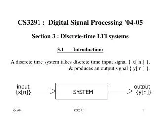
CS3291 : Digital Signal Processing '04-05 Section 3 : Discrete-time LTI systems 3.1 Introduction: A discrete time system takes discrete time input signal { x[ n ] }, & produces an output signal { y[ n ] }.

E N D
CS3291 : Digital Signal Processing '04-05 Section 3 : Discrete-time LTI systems 3.1 Introduction: A discrete time system takes discrete time input signal { x[ n ] }, & produces an output signal { y[ n ] }. CS3291
Implemented by general purpose computer, microcomputer or dedicated digital hardware capable of carrying out arithmetic operations on samples of {x[n]} and {y[n]}. • {x[n]} is sequence whose value at t=nT is x[n]. • Similarly for {y[n]}. • T is sampling interval in seconds. • 1/T is sampling frequency in Hz. • {x[n-N]} is sequence whose value at t=nT is x[n-N].{x[n-N]} is {x[n]} with every sample delayed by N sampling intervals. • Many types of discrete time system can be considered, e.g. CS3291
A x[n] y[n] • (i) Discrete time "amplifier" with output: • y[n] = A . x[n]. • Described by "difference equation": y[n] = A x[n]. • Represented in diagram form by a "signal flow graph” . CS3291
(ii) Processing system whose output at t=nT is obtained by weighting & summing present & previous input samples: y[n] = A0 x[n] + A1 x[n-1] + A2 x[n-2] + A3 x[n-3] + A4x[n-4] ‘Non-recursive difference equatn’ with signal flow graph below. Boxes marked " z -1 " produce a delay of one sampling interval. CS3291
(iii) System whose output y[n] at t = nT is calculated according to the following recursive difference equation: • y[n] = A 0 x[n] - B 1 y[n-1] • whose signal flow graph is given below. • Recursive means that previous values of y[n] as well as present & previous values of x[n] are used to calculate y[n]. A0 y[n] x[n] z-1 B1 CS3291
(iv) A system whose output at t=nT is: y[n] = (x[n]) 2 as represented below. y[n] x[n] CS3291
3.2. LTI Systems: • To be LTI, a discrete-time system must satisfy: • (I) Linearity ( Superposition ): • Given any two discrete time signals {x 1 [n]} & {x 2 [n]}, • if {x 1 [n]}{y 1 [n]} & {x 2 [n]}{y 2 [n]} • then for any values of k 1 and k 2, • response to k 1{x 1[n]} + k 2{x 2[n]} • must bek 1{y1[n]} + k 2{y 2 [n]} . • To multiply a sequence by k, multiply each element by k, • k{x[n]} = {k x[n]}. • To add two sequences together, add corresponding samples, • {x[n]} + {y[n]} = {x[n] + y[n]}.) CS3291
(II) Time-invariance : • Given any discrete time signal {x[n]}, • if response to {x[n]} is {y[n]}, • response to {x[n-N]} must be {y[n-N]} for any N. • Delaying input by N samples only delays output by N samples. • Examples (i), (ii) and (iii) are LTI whereas (iv) is not LTI . CS3291
3.3. Impulse-response: Useful to consider response of LTI systems to a discrete time unit impulse , or in short an impulse denoted by {d [n] } with: CS3291
{d[n-N]} is delayed impulse where the only non-zero sample occurs at n=N rather than at n=0. • When input is {d[n]}, output is impulse response {h[n]}. • If impulse-response of an LTI system is known, its response to any other input signal may be predicted. CS3291
X3 X1 X4 X2 X5 - 1 - 1 - 1 - 1 z z z z x[n] A3 A4 A5 A2 A1 Y y[n] • 3.4. Computing an impulse response: • Consider a discrete time system with signal-flow graph below with A1, A2, A3, A4, A5 set to specific constants. • Notice the labels X1, X2, etc. • Realised by microcomputer running a program with flow-diagram & high-level language implementation as listed next. CS3291
clear all; A1=1; A2=2; A3=3; A4=-4; A5=5; x1=0; x2=0; x3=0; x4=0; x5=0; while ~isempty(X) X = input( 'X = '); x1 = X; Y= A1*x1 + A2*x2 + A3*x3 + A4*x4 + A5*x5 ; disp([' Y = ' num2str(Y)]); x5 = x4 ; x4 = x3; x3 = x2 ; x2 =x1; end; % MATLAB program Set A1,A2,…. Zero X1, X2, X3, X4,X5 INPUT X Y = A1*X + A2*X2 + A3*X3 +... OUTPUT Y X5 = X4; X4 = X3; X3 = X2; X2 =X1 CS3291
Here is another version using MATLAB arrays: A = [1 2 3 -4 5 ] ; x = [0 0 0 0 0 ] ; while 1 X = input( 'X = '); x(1)=X; Y=A(1) * X; for k = 2 : 5 Y = Y + A(k)*x(k); end; disp([' Y = ' num2str(Y)]); for k=5:-1:2 x(k) = x(k-1); end; end; CS3291
And an even more efficient version A = [1 2 3 -4 5 ] ; x = [0 0 0 0 0 ] ; while 1 x(1) = input( 'X = '); Y = A(1)*x(1); for k = 5 : -1: 2 Y = Y + A(k)*x(k); x(k) = x(k-1); end; disp([' Y = ' num2str(Y)]); end; CS3291
These can be run in MATLAB • The ‘while 1’ statement initiates an infinite loop. • Program will run for ever • or until interrupted by ‘CONTROL+C’ CS3291
Impulse-response for this example may be deduced by running program & entering values for X on the keyboard : • 0, 0, 0, 1, 0, 0, 0, 0,.... • Sequence of output samples printed out will be : • 0, 0, 0, A1, A2, A3, A4, A5, 0, 0, .... • Impulse-response can also be obtained by tabulation (later). • Output must be zero until input becomes equal to 1 at n=0 • Impulse response is: • {..., 0, ..., 0, A1, A2, A3, A4, A5, 0, 0, ... ,0,...} • where the sample at n=0 is underlined. • Only five non-zero output samples are observed. • This is a " finite impulse-response ” (FIR). CS3291
Exercise 3.1: • Calculate impulse-responses for difference equations: • (i) y[n] = x[n] + 2 x[n-1] + 3 x[n-2] - 4 x[n-3] + 5 x[n-4] • (ii) y[n] = 4 x[n] - 0.5 y[n-1] • Solutions: • If computer not available we may use a tabulation. • Difference eqn (i) will produce a finite impulse-response. • Difference eqn (ii) produces infinite response whose samples gradually reduce in amplitude but never quite become zero. CS3291
(i) y[n] = x[n] + 2 x[n-1] + 3 x[n-2] - 4 x[n-3] + 5 x[n-4] n x[n] x[n-1] x[n-2] x[n-3] x[n-4] y[n] -1 0 0 0 0 0 0 0 1 0 0 0 0 1 1 0 1 0 0 0 2 2 0 0 1 0 0 3 3 0 0 0 1 0 -4 4 0 0 0 0 1 5 5 0 0 0 0 0 0 :::::: : Solution is:- {.. 0, .., 0, 1, 2, 3, -4, 5, 0, .., 0, ...} CS3291
Difference equation (ii): y[n] = 4 x[n] - 0.5 y[n-1] n x[n] y[n-1] y[n] 0 1 0 4 1 0 4 -2 2 0 -2 1 3 0 1 -0.5 4 0 -0.5 0.25 5 0 0.25 -0.125 :: : : Solution is: {.., 0, .., 0, 4, -2, 1, -0.5, 0.25, -0.125, ...) CS3291
3.5. Digital filters: • A "digital filter” is a digitally implemented LTI discrete time system governed by a difference equation of finite order; e.g. : • (i) y[n] = x[n] + 2 x[n-1] + 3 x[n-2] - 4 x[n-3] + 5 x[n-4] • (ii) y[n] = 4 x[n] - 0.5 y[n-1] • Difference equation (i) is "non-recursive" • & produces a finite impulse response (FIR). • Difference equation (ii) is " recursive " . • Impulse-response of a recursive difference equation can have an infinite number of non-zero terms. • In this case it is an infinite impulse-response (IIR). CS3291
Next slide has yet another way of programming difference equations (i.e. digital filters) in MATLAB. • But this time, we use a MATLAB function and operate on a whole array of music at once. • You can find the music file ‘cap4th.wav’ in • www.cs.man.ac.uk/~barry/mydocs/CS3291/MATLAB CS3291
MATLAB function ‘filter’ used for non-recursive diffce eqn y = filter(A, 1, x) filters signal in array x to create array y. For each sample x(n) of array x: y(n) = A(1)*x(n) + A(2)*x(n-1) + ... + A(N+1)*x(n-N) Example (i): y[n] = x[n] + 2 x[n-1] + 3 x[n-2] - 4 x[n-3] + 5 x[n-4] [x, fs, nbits] = wavread ('cap4th.wav'); sound(x,fs,nbits); pause; y = filter ( [1 2 3 -4 5], 1, x); sound(y,fs,nbits); CS3291
Use of ‘filter’ for recursive difference equatn y = filter(A, B, x) filters signal in array x to create array y using a recursive difference equation. Example (ii): y[n] = 4 x[n] - 0.5 y[n-1] [x, fs, nbits] = wavread ('cap4th.wav'); sound(x,fs,nbits); pause; y = filter ( [4], [1 0.5], x); sound(y,fs,nbits); CS3291
3.6. Discrete time convolution: If impulse-response of an LTI system is {h[n]} its response to any input {x[n]} is an output {y[n] } whose samples are given by the following "convolution" formulae: Consider the response of a system with impulse response: {h[n]} = { ..., 0,..., 0, 1, 2, 3, -4, 5, 0, .....0, .... } to {x[n]} = { ... 0, ... , 0 , 1, 2, 3, 0, ..., 0, ....} CS3291
Result is not too surprising. • It is the difference equation for an LTI system whose impulse response is {.., 0, .., 0, 1, 2, 3, -4, 5, 0, .., 0, ..}. • Program discussed earlier implements this difference equation, • We could complete the example by running it, entering samples of • { x[n] }, and noting the output sequence. • Alternatively, we could use tabulation as follows: CS3291
y[n] = x[n] + 2x[n-1] + 3x[n-2] - 4x[n-3] + 5x[n-4] n x[n] x[n-1] x[n-2] x[n-3] x[n-4] y[n] : : : : : : : -1 0 0 0 0 0 0 0 1 0 0 0 0 1 1 2 1 0 0 0 4 2 3 2 1 0 0 10 3 0 3 2 1 0 8 4 0 0 3 2 1 6 5 0 0 0 3 2 -2 6 0 0 0 0 3 15 7 0 0 0 0 0 0 : : : : : : : {y[n]} = { .... 0, ....., 0, 1, 4, 10, 8, 6, -2, 15, 0, ...., 0, ....} CS3291
3.7. Proof of discrete time convolution formulae: Only use defns of linearity, time-invariance & impulse-response. Since d[n-m] is non-zero only at n = m, given any sequence {x[n]}, {x[n]} is sum of infinite number of delayed impulses{d[n-m]} each multiplied by a single element, x[m]. Response to {d[n-m]} is {h[n-m]} for any value of m. response to {x[n]} is : CS3291
h[n] x[n] 3 2 2 n n • Replacing n-m by k gives the alternative formula. • Study the graphical explanation of this proof in Section 3.17. {x[n]} = { ..., 0, ..., 0, 1, 2, 3, 0, 0, ..., 0, ...} {h[n]} = { ..., 0, ..., 0, 1, 2, 1, 2, 0, ..., 0...} CS3291
x[n] 3 2 d[n] h[n] n 2 n n 2d[n-1] 2h[n-1] 4 2 2 n n 3d[n-2] 3h[n-2] 6 3 3 n n 3.17 Discrete time convolution graphically {h[n]} = { ..., 0, ..., 0, 1, 2, 1, 2, 0, ..., 0,...} {x[n]} = { ..., 0, ..., 0, 1, 2, 3, 0, 0, ..., 0, ...} CS3291
y[n] 10 8 6 4 2 n Express: {x[n]} = {d[n]} + 2 {d[n-1]} + 3 {d[n-2]} Response is: {y[n]} = {h[n]} + 2 {h[n-1} + 3 {h[n-2]} CS3291
y[n] x[n] 10 8 3 6 2 4 2 n n {h[n]} = { ..., 0, ..., 0, 1, 2, 1, 2, 0, ..., 0,...} {x[n]} = { ..., 0, ..., 0, 1, 2, 3, 0, 0, ..., 0, ...} { d[n] } {h[n]} + 2{ d[n-1 ]} + 2 { h[n-1]} + 3 { d[n-2] } + 3 { h[n-2] } CS3291
d[n] h[n] 2 n n 2h[n-1] 4 2 n 3d[n-2] 3h[n-2] 6 3 3 n n 2d[n-1] 2 n CS3291
3.8. Stability: An LTI system is stable if its impulse-response {h[n]} satisfies: This means that {h[n]} must be either an FIR or an IIR whose samples decay towards zero as n . 3.9. Causality: An LTI system operating in real time must be "causal " which means that its impulse-response {h[n]} must satisfy: h[n] = 0 for n < 0. Non-causal system would need “crystal ball ” to predict future. CS3291
3.10. Relative Frequency • Study effect of digital filters on sine-waves of different frequencies. • Discrete time sine-wave obtained by sampling A cos(t + ). • If sampling period is T seconds, resulting discrete time signal is : • = T is “ relative" frequency of sampled sine-wave. • Units of are 'radians per sample'. • To convert back to true frequency (radians/s ) multiply by 1/T. • Note: 1/T = sampling frequency, f S, in samples/second (Hz). • ‘radians / sample’ times ‘samples / second’ = ‘radians / second’ • Normally process analogue signals in range 0 to f S /2 ( = 1/(2T) ), • Restricts to the range 0 to . CS3291
cos( t ) =2 / (8T) t -4T -3T 3T 4T -T T cos( T n ) = 2 / 8 n -4 -3 3 4 -1 1 CS3291
Table gives values of & corresponding true frequencies :- Relative frequency True frequency (radians/sample) (radians/s) (Hz) 0 0 0 /6 fS/6 fS/12 /4 fS/4 fs/8 /3 fS/3 fs/6 /2 fS/2 fs/4 2/3 2fS/3 fs/3 fSfS/2 ‘radians / sample’ ‘samples / second’ = ‘radians / second’ CS3291
3.11. Relative frequency response Response to sampled sine-waves calculated by defining: If this is applied to a system with impulse response {h[n]}, output would be {y[n]} with : CS3291
cos( (2/8) n ) -4 -3 3 4 -1 1 n sin( (2/8) n) n -2 -1 1 3 CS3291
H( e j ) is the " relative frequency response " of LTI system. • Complex number for any value of . • It is DTFT of { h[n] }. • Note similarity to the analogue Fourier transform. CS3291
If input is {e j n }, output is same sequence with each element multiplied by H( e j ). { e j n H(e j n ) } {e j n } LTI {h[n]} • When { h[n] } is real, H( e -j ) = H*( e j ). • Exercise: Prove this. CS3291
Remember the analogue case:- e j t Ha(j ) e j t LTI ha(t) • When h(t) is real, Ha(j ) = Ha*(j ) CS3291
3.12. Gain and phase responses • Expressing H( e j ) = G() e j () • G() = |H( e j )| is "gain ” • () = arg ( H( e j ) ) is "phase lead”. • Both vary with . • If input is {A cos(n)}, • output is: { G()A cos(n + ()) } • Exercise: Prove this • When input is sampled sine-wave of rel frequency , output is sine-wave of same frequency , but with amplitude scaled by G() & phase increased by (). CS3291
Gain & phase response graphs again 20log10[G()] dB -() -() G() in dB 0 /4 /2 3/4 CS3291
Common to plot graphs of G() & () against . • G() often converted to dBs by calculating 20 log10( G() ). • Restrict to lie in range 0 to & adopt a linear horizontal scale. • Example 3.2: • Calculate gain & phase response of FIR digital filter in Figure 3.3 where A1 = 1, A2 = 2, A3 = 3, A4 = -4, A5 = 5 . • Solution: • Impulse response is: {.., 0, .., 0, 1, 2, 3, -4, 5 ,0, .., 0,..}. • By the formula established above, • H( e j ) = 1 + 2 e - j + 3 e -2 j - 4 e -3 j + 5 e - 4 j • To obtain the gain and phase at any take modulus and phase. • Best done by computer, either by writing & running a simple program, or by running a standard package. • A simple program is given at the end of these notes. CS3291
Can use a spread-sheet such as excel (see lecture notes) • Another way of calculating gain & phase responses for • H( e j ) = 1 + 2 e - j + 3 e -2 j - 4 e -3 j + 5 e - 4 j • is to start MATLAB and type: • A = [ 1 2 3 -4 5 ]; • freqz( A ); • See later section 3.18 for graphs produced. CS3291
Produces graphs of gain & phase responses of H( ej). • Frequency scale normalised to fS/2 & labelled 0 to 1 • instead of 0 to . • See Section 3.18 • In next section we calculate coeffs of an FIR filter to achieve a particular type of gain & phase response. • To calculate gain & phase responses for an IIR filter would be difficult by method used above because impulse-response has infinite number of non-zero terms. • There is an easier method in a later section. CS3291
Phase delay • Assume input is {A cos(n)}, • Output is: { G() A cos ( n + () ) } • = { G() A cos ( [ n + () / ])} • ={ G() A cos ( [ n - (-() / ) ]) } • Phase lead () delays sine-wave by -()/sampling intervals • This is ‘phase-delay’. CS3291
3.13. Linear phase response • If -()/ remains constant for all values of , • i.e. if -() = k for constant k, • system has ‘linear phase’ response. • Graph of -() against on linear scale would then be • straight line with slope k where k is "phase delay" • i.e. the delay measured in sampling intervals. • This need not be an integer. CS3291
-()/ -() -()/ G() in dB 0 /4 /2 3/4 Gain, phase & ‘phase-delay’ response graphs Not ‘linear-phase’. CS3291
Gain, phase & ‘phase-delay’ response graphs again -()/ -() -()/ k G() in dB 0 /4 /2 3/4 This is ‘linear-phase’ as -()/ is constant. CS3291