Download
1 / 30
300 likes | 434 Views
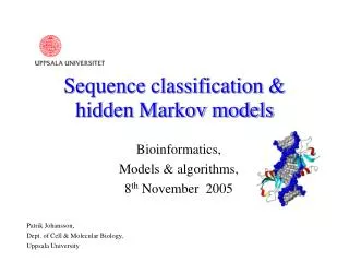
Bioinformatics, Models & algorithms, 8 th November 2005 Patrik Johansson, Dept. of Cell & Molecular Biology, Uppsala University. Sequence classification & hidden Markov models. A family of proteins share a similar structure but not necessarily sequence.

E N D
Bioinformatics, Models & algorithms, 8th November 2005 Patrik Johansson, Dept. of Cell & Molecular Biology, Uppsala University Sequence classification & hidden Markov models
A family of proteins share a similar structure but not necessarily sequence
Classification of an unknown sequence s to family A or B using HMMs A A A A A A A A A s B B B B B B B B
A A A B B B C C C Hidden Markov Models, introduction • General method for pattern recognition, comp. Neural networks • An HMM generates sequences / sequence distributions • Markov chain of events Three coins A, B & C gives a Markov chain Г = CAABA.. Outcome, e.g. Heads Heads Tails, generated by hidden Markov chain Г
A A A B B B C C C Heads Tails Tails Hidden Markov Models, introduction.. • Model M is emitting a symbol (T, H) in each state i based on some probability ei • The next state j is chosen based on some transition probability ai,j e.g, the sequence s = ‘Tails Heads Tails’ over the pathГ = BCC
B E M1 Mj MN Profile hidden Markov Model architecture • A first approach for sequence distribution modelling
Ij B E Mj - Mj Mj+ Profile hidden Markov Model architecture.. • Insertion modelling Insertions random; ejI(a) =q(a)
Mj Dj Mj Profile Hidden Markov Model architecture.. • Deletion modelling Alt.
Profile Hidden Markov Model architecture.. Insert & deletestates are generalized to all positions. The model M can generate sequences from state B by successive emissions and transitions to state E Dj Ij E B Mj
Probabilistic sequence modelling • Classification criteria ( 1 ) Bayes theorem ; ( 2 ) ..but, P(M) & P(s)..? ( 3 )
Probabilistic sequence modelling.. If N models the whole sequence space (N = q) ( 4 ) Since , logarithm probabilities more convenient Def., log-odds score V; ( 5 )
Probabilistic sequence modelling.. Eq. ( 4 ) & ( 5 ) gives new classification criteria ; logzP(s | M) ≥ d ( 6 ) score = logzP(s | q) ..for a certain significance level (i.e. the number of incorrect classifications in an n big database) a threshold d is required ( 7 )
Probabilistic sequence modelling.. Example If z=e or z=2, the significance level is chosen to one incorrect classification (false positive) per 1000 trials in a database of n=10000 sequences ; bits nits,
Large vs. small threshold d High d A Low d A A A A A A A A B B B B B True positives B B B False positive
Model characteristics One can define sensitivity, ‘how many are found’ ; ..and selectivity, ‘how many are correct’ ;
Model construction • From initial alignment Most common method. Start from an initial multiple alignment of e.g. a protein family • Iteratively By successive database searches incorporating new similar sequences into the model • Neural-inspired The model is trained using some continuous minimization algorithm, e.g. Baum-Welsh, Steepest Descent etc.
E Model construction.. A short family alignment gives a simple model M, potential matchstates marked with an () B
E B E B E B B E Model construction.. A more generalized model Ex. evaluate sequence s=‘AIEH’
Dj-1 Ij-1 Mj-1 Mj Sequence evaluation The optimal alignment, i.e. the path that has the greatest probability of generating sequences s, can be determined through dynamic programming The maximum log-odds score VjM(si) for matchstate j that is emitting si is calculated from the emission score, previous maximum score plus transition score
Sequence evaluation.. Viterbis Algorithm, ( 8 ) ( 9 ) ( 10 )
Parameter estimation, background • Proteins with similar structures can have very different sequences • Classical sequence alignment based only on heuristic rules & parameters cannot deal with sequence identities below ~ 50-60% • Substitution matrices add static a priori information about amino acids and protein sequences good alignments down to ~ 25-30% sequence identity, ex. CLUSTAL • How to get further down into ‘the twilight zone’..? - More and dynamic a priori information..!
Parameter estimation Probability of emitting an alanine in the first matchstate, eM1(‘A’)..? • Maximum likelihood-estimation
Parameter estimation.. • Add-one pseudocount estimation • Background pseudocount estimation
Parameter estimation.. • Substitution mixture estimation Score : Maximum likelihood gives pseudocounts : Total estimation :
Parameter estimation.. All above methods are in spite of their dynamic implementation, still based on heuristic parameters Method that compensates & complements lack of data in a statistically correct way ; • Dirichlet mixture estimation Looking at sequence alignments, several different amino acid distributions seem to be reoccurring, not just the background distribution q Assume that there are k probability densities that generates these
Parameter estimation, Dirichlet Mixture style.. Given the data, a countvector , this method allows a linear combination of k individual estimations weighted with the probability that n is generated by each component The k componets can be modelled from a curated database of alignments. Using some parametric form of the probability density, an explicit expression for the probability that n has been generated by the jth component can be derived Ex.
Parameter estimation, Dirichlet Mixture style.. n The k components describe peaks of aa distributions in some kind of multidimensional space Depending on where in sequence space our countvector n lies, i.e. depending on which components that can be assumed to have generatedn, distribution information is incorporated into the probability estimation e
Classification example Alignment of some known glycoside hydrolase family 16 sequences • Define which columns are to be regarded as matchstates (*) • Build the corresponding model M & HMM graph • Estimate all emission and transition probabilities, ej& ajk • Evaluate the log-odds score / probability that an unknown sequence s has been generated by M using Viterbis algorithm • If score(s | M) > d, the sequence can be classified as a GH16 family member
Classification example.. A certain sequence s1=WHKLRQ.. is evaluated and gets a score of -17.63 nits, i.e. the probability that M has generated s1 is very small Another sequence s2=SDGSYT.. gets a score of 27.49 nits and can with good significance be classified as a family member
Summary • Hidden Markov models are used mainly for classification / searching (PFAM), but also for sequence mapping / alignment • As compared to normal alignment, a position specific approach is used for sequence distributions, insertions and deletions • Model building is usually a compromise between sensitivity and selectivity. If more a priori information is incorporated, the sensitivity goes up whereas the selectivity goes down