Introducing Duality and Sensitivity Analysis

1. Introducing Duality and Sensitivity Analysis

2. Merton Trucks Optimal Product Mix: 2000 Model 101s and 1000 Model 102s Optimal Contribution: $11,000,000 How much is Engine Assembly capacity worth to Merton Trucks?

3. Merton Trucks (Scaled) unit = 1 hr unit = 2 hr unit = 2 hr unit = 3 hr Optimal Product Mix: 2000 Model 101s and 1000 Model 102s Optimal Contribution: $11,000,000 How much is Engine Assembly capacity worth to Merton Trucks?

4. Worth of Engine Capacity

5. Suppose now, that the engine assembly capacity increases to 4400 hours

6. Worth of Engine Capacity Engine Assembly Capacity is now 4400 hours

7. Worth of Engine Capacity Engine Assembly Capacity is now 4400 hours

8. Worth of Engine Capacity Engine Assembly Capacity is now 4400 hours

9. Worth of Engine Capacity Engine Assembly Capacity is now 4400 hours

10. Worth of Engine Capacity Engine Assembly Capacity is now 4400 hours

11. Merton Trucks Base Engine Assembly capacity = 4000 hrs Engine Assembly capacity = 4000 hrs

12. Merton Trucks Base Engine Assembly capacity = 4000 hrs Engine Assembly capacity ↑ by 1%

13. Merton Trucks Base Engine Assembly capacity = 4000 hrs Engine Assembly capacity ↑ by 5%

14. Merton Trucks Base Engine Assembly capacity = 4000 hrs Engine Assembly capacity ↑ by 10%

15. Merton Trucks (new) Base Engine Assembly capacity = 4400 hrs Engine Assembly capacity = 4400 hrs

16. Merton Trucks (new) Base Engine Assembly capacity = 4400 hrs Engine Assembly capacity ↑ by 1%

17. Merton Trucks (new) Base Engine Assembly capacity = 4400 hrs Engine Assembly capacity ↑ by 5%

18. Merton Trucks (new) Base Engine Assembly capacity = 4400 hrs Engine Assembly capacity ↑ by 10%

19. Forming the dual Input (Primal): • Maximization objective • Non-negative decision variables • “Less than or equal to” type constraints Output (Dual): • Minimization objective • One dual variable for each primal constraint • Non-negative dual variables • “Greater than or equal to” type constraints • One constraint for each primal variable

20. Some Laws • The objective function values of optimal solutions to primal and dual problems are equal. • If there is excess of a resource at an optimal solution, then its shadow price is zero. • If the shadow price of a resource is positive, then it has got completely used up at an optimal solution. • It is possible for a resource to get completely used up at an optimal solution and still have a zero shadow price.

21. Reduced Costs The reduced cost of a coefficient of a decision variable in the objective function is the minimum amount by which the coefficient should be reduced in order that the decision variable achieves a non-zero level in an optimal solution. • The reduced cost for a decision variable already at non-zero value in an optimal solution is ZERO. • For a minimization problem, reduced costs are either ZERO or POSITIVE. • For a maximization problem, reduced costs are either ZERO or NEGATIVE. • A decision variable at zero level can have a reduced cost of zero.

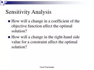
22. Sensitivity Analysis Sensitivity analysis tells us what changes are possible in the coefficients of a linear programming model without changing the optimal basis. • We are concerned with changing only one coefficient and keeping all others fixed. • We are bothered only about the set of constraints that define the optimal solution – they should not change. Otherwise, the optimal solution can change, the objective function value can change.

23. Sensitivity Analysis Optimum Value = 11 Million Model_101 = 2000 Model_102 = 1000 Original Model

24. Sensitivity Analysis Optimum Value = 13 Million Model_101 = 2000 Model_102 = 1000 Objective function coefficient increases Z = 3000 Model_101 + 5000 Model_102 to Z = 4000 Model_101 + 5000 Model_102

25. Sensitivity Analysis Optimum Value = ??? Model_101 = 2000 Model_102 = 1000 Objective function coefficient increases Z = 3000 Model_101 + 5000 Model_102 to Z = 6000 Model_101 + 5000 Model_102

26. Sensitivity Analysis Optimum Value = 17.5 Million Model_101 = 2000 Model_102 = 1000 Objective function coefficient increases Z = 3000 Model_101 + 5000 Model_102 to Z = 6000 Model_101 + 5000 Model_102

27. Sensitivity Analysis Optimum Value = 11 Million Model_101 = 2000 Model_102 = 1000 Original Model

28. Sensitivity Analysis Optimum Value = 10.5 Million Model_101 = 2000 Model_102 = 1000 Objective function coefficient decreases Z = 3000 Model_101 + 5000 Model_102 to Z = 2750 Model_101 + 5000 Model_102

29. Sensitivity Analysis Optimum Value = ??? Model_101 = 2000 Model_102 = 1000 Objective function coefficient decreases Z = 3000 Model_101 + 5000 Model_102 to Z = 2000 Model_101 + 5000 Model_102

30. Sensitivity Analysis Optimum Value = 9.5 Million Model_101 = 2000 Model_102 = 1000 Objective function coefficient decreases Z = 3000 Model_101 + 5000 Model_102 to Z = 2000 Model_101 + 5000 Model_102

31. Sensitivity Analysis Objective function coefficient change

32. Sensitivity Analysis Optimum Value = 11 Million Model_101 = 2000 Model_102 = 1000 Original Model

33. Sensitivity Analysis Optimum Value = 11.4 Million Model_101 = 1800 Model_102 = 1200 Engine Assy. RHS increases Model_101 + 2 Model_102 ≤ 4000 to Model_101 + 2 Model_102 ≤ 4200

34. Sensitivity Analysis Optimum Value = 12 Million Model_101 = 1500 Model_102 = 1500 Engine Assy. RHS increases Model_101 + 2 Model_102 ≤ 4000 to Model_101 + 2 Model_102 ≤ 4600

35. Sensitivity Analysis Optimum Value = 11 Million Model_101 = 2000 Model_102 = 1000 Original Model

36. Sensitivity Analysis Optimum Value = 10.6 Million Model_101 = 2200 Model_102 = 800 Engine Assy. RHS decreases Model_101 + 2 Model_102 ≤ 4000 to Model_101 + 2 Model_102 ≤ 3800

37. Sensitivity Analysis Optimum Value = 9 Million Model_101 = 2500 Model_102 = 300 Engine Assy. RHS decreases Model_101 + 2 Model_102 ≤ 4000 to Model_101 + 2 Model_102 ≤ 3100

38. Sensitivity Analysis Engine Assy. RHS change