Download

1 / 39
390 likes | 476 Views
Analysis and Optimization of Fault-Tolerant Embedded Systems with Hardened Processors. Ilia Polian Institute for Computer Science, Albert-Ludwigs-University of Freiburg, Germany. Paul Pop Dept. of Informatics and Mathematical Modeling Technical University of Denmark (DTU), Denmark.

E N D
Analysis and Optimization of Fault-Tolerant Embedded Systems with Hardened Processors Ilia Polian Institute for Computer Science, Albert-Ludwigs-University of Freiburg, Germany Paul Pop Dept. of Informatics and Mathematical Modeling Technical University of Denmark (DTU), Denmark Viacheslav Izosimov, Petru Eles, Zebo Peng Embedded Systems Lab (ESLAB), Linköping University, Sweden
Motivation • Hard real-time safety-critical applications • Time-constrained • Cost-constrained • Quality-of-service • Fault-tolerant • etc. • Focus ontransient faults and intermittent faults
Transient and Intermittent Faults Electromagneticinterference (EMI) Internal EMI Crosstalk Radiation Power supplyfluctuations Lightning storms Software errors(Heisenbugs) Errors caused by transient (intermittent)faults have to be tolerated beforethey crash the system
Hardening • Hardening • Improving the hardware architecture to reduce the error rate • Hardware redundancy (selective duplication of gates/units/nodes, dedicated additional hardware modules/flip-flops) • Re-designing the hardware to reduce susceptibility to transient faults • Using higher voltages / lower frequencies / larger transistor sizes • Protecting with shields • Lead to lower performance • Use of technologies few generations back • Increase of the critical path and silicon area • Very expensive • Extra-design effort / More expensive technologies • More silicon / Increase in the number of gates or computation units • Low production volumes • Still may not guarantee the required reliability levels at affordable cost!
Software-level Fault Tolerance • Software fault tolerance • Reliability increase with time redundancy • Lead to lower performance • Fault tolerance overheads • Overheads due to error detection, voting, agreement • Low hardware cost • Often cannot guarantee the required reliability levels and, at the same time, meet deadlines! P1 P1 P1
Motivation Fault tolerance against transient faults may lead to significant performance or cost overhead! Neither hardening nor pure software-level fault tolerance can guarantee the required level of reliability… A trade-off between hardware and softwarefault tolerance has to be addressed to providea reliable and low-cost system!
Outline • Motivation • Architecture • Application example • Fault tolerance: hardening & re-execution • Hardening/re-execution trade-off • Problem formulation & design strategy • Experimental results • Conclusions
Transient faults Processes: Re-execution Computation nodes: Hardening Messages: Fault-tolerant predictable protocol P5 m2 m1 P1 P2 P3 P4 Architecture … The error rates for each hardening version (h-version) of each computation node The reliability goal = 1 is the maximum probability of a system failure due to transient faults on any computation node within a time unit
= 1 10-5 N1 h = 2 h = 3 h = 1 N1 Increase in reliability Decrease in process failure probabilities p t p t p t Cost is increasedwith more hardening! P1 80 4·10-2 4·10-4 160 100 4·10-6 Hardening versions of computation node N1 Worst-case execution times are increased Hardening performance degradation (HPD) Cost 10 20 40 Application Example P1 t – worst-case execution time p – process failure probability Cost – h-version cost
System Failure Probability (SFP) Analysis We have proposed a system failure probability (SFP) analysis to connect error rates and the reliability goal to the number of re-executions in software h = 1 N1 = 1 10-5 t p T = 360ms 4·10-2 P1 80 Non-trivial Exact Safe SFP main execution + k = 6 re-executions
System Failure Probability (SFP) Analysis We have proposed a system failure probability (SFP) analysis to connect error rates and the reliability goal to the number of re-executions in software h = 2 N1 = 1 10-5 t p T = 360ms 4·10-4 P1 100 SFP main execution + k =2 re-executions
System Failure Probability (SFP) Analysis We have proposed a system failure probability (SFP) analysis to connect error rates and the reliability goal to the number of re-executions in software h = 3 N1 = 1 10-5 t p T = 360ms 4·10-6 P1 160 SFP main execution + k =1 re-executions
= 1 10-5 N1 h = 2 h = 3 h = 1 N1 p t p t p t = 20 ms P1 80 4·10-2 4·10-4 160 100 4·10-6 D = 360ms Cost 10 20 40 N1 1 P1/1 P1/2 P1/3 P1/4 P1/5 P1/6 P1/7 N1 2 P1/1 P1/2 P1/3 N1 3 P1/1 P1/2 Application Example
h = 2 h = 3 h = 1 h = 2 h = 3 h = 1 N1 N2 p p t p t p t t p t p t 50 P1 P1 1·10-3 60 90 1.2·10-10 75 1.2·10-3 1.2·10-5 60 75 1·10-10 1·10-5 65 P2 1.2·10-3 1.3·10-5 105 1.3·10-10 P2 90 75 1.3·10-3 1.2·10-5 1.2·10-10 75 90 90 50 1.2·10-3 1.4·10-5 1.4·10-10 75 60 75 1.2·10-10 P3 60 1.2·10-5 P3 1.4·10-3 90 1.6·10-5 105 1.6·10-10 90 1.3·10-10 1.6·10-3 75 1.3·10-5 P4 75 65 P4 1.3·10-3 Cost Cost 16 32 64 20 40 80 Application Example D = 360 ms P1 P3 N1 N2 m3 m1 m4 = 15 ms m2 P2 P4 = 1 10-5
P1 P2/1 P2/2 N1 2 N2 P3/1 P3/2 P4 2 bus m3 m2 N1 2 P1 P3 P2/1 P2/2 P4/1 P4/2 N2 2 P1 P3 P2/1 P2/2 P4/1 P4/2 P4 N1 P1 P3 P2 3 N2 3 P1 P3 P2 P4 Application Example Ca = 32 Cb = 40 Cc = 64 Cd = 80 Ce = 72
Problem Formulation (Input) Input: • Application as a set of directed acyclic graphs • Reliability goal • Deadline D, period T • Recovery overhead • Bus-based hardware architecture • Process worst-case execution times for all h-versions of computation nodes • Process failure probabilities for all h-versions • Costs of all h-versions • Worst-case message sizes, transformed into the worst-case transmission times on the bus
Problem Formulation (Output) Output: • Selection of h-versions of computation nodes • Mapping of all processes • Maximum number of re-executions (by using our SFP analysis) • Schedule (static cyclic) of all processes and messages • The final solution has to • Be schedulable • Meet reliability goal • Minimize the overall system cost
Design Optimization Strategy Satisfy Reliability Input: Reliability Goal Period T Process Failure Probabilities Mapping + Hardening Setup SFP Number ofRe-executions Re-executionOptimization (based on SFP)
Design Optimization Strategy Meet Deadline Satisfy Reliability SFP Input: Reliability Goal Period T Process Failure Probabilities Mapping HardeningSetup Number ofRe-executions Re-executionOptimization (based on SFP) HardeningOptimization + Scheduling
Design Optimization Strategy Meet Deadline Meet Deadline Satisfy Reliability SFP Input: Reliability Goal Period T Architecture (Set of Nodes) Selection HardeningSetup Number ofRe-executions Mapping Re-executionOptimization (based on SFP) MappingOptimization + Scheduling HardeningOptimization + Scheduling
Design Optimization Strategy BestCost Meet Deadline Meet Deadline Satisfy Reliability SFP HardeningSetup Number ofRe-executions Mapping ArchitectureSelection Re-executionOptimization (based on SFP) MappingOptimization + Scheduling HardeningOptimization + Scheduling ArchitectureOptimization DATE’05
MAX MIN OPT 100 80 60 % accepted architectures 40 20 0 10-12 10-11 10-10 Selected Experimental Results MAX – hardware optimization MIN – software optimization OPT – combined architecture Accepted architecture: Satisfying maximum accepted cost Satisfying reliability goal Schedulable Hardening performance degradation (HPD) 5% Performance difference between the least hardened and the most hardened versions Maximum cost 20 % accepted architectures as a function ofsoft error rate (SER)
Selected Experimental Results 100 MAX MIN OPT 80 60 % accepted architectures 40 20 0 10-12 10-11 10-10 MAX – hardware optimization MIN – software optimization OPT – combined architecture Hardening performance degradation (HPD) 100% Maximum cost 20 % accepted architectures as a function ofsoft error rate (SER)
Combining hardware and software fault tolerance techniques is essential for obtaining cost efficient implementation of fault-tolerant embedded systems Conclusions • Design optimization strategy for minimization of overall system cost by trading-off between hardening and re-execution • Hardware + software fault tolerance techniques • System failure probability (SFP) analysis • A set of design optimization heuristics
System Failure Probability (SFP) Analysis Given: • Application as a set of directed acyclic graphs, period T • Reliability goal • Architecture composed of a set of h -versions of computation nodes • Mapping of processes on the nodes • Process failure probabilities for all h –versions • The number of re-executions kj on each node Nj Output: • True,if the system reliability is above or equal to the reliability goal • False, if the system reliability is below the reliability goal
System Failure Probability (SFP) Analysis Probability of a system failure during period T due to transient faults, or the probability that any of Nj nodes experience more than kj transient faults during period T ( is time unit for reliability goal )
System Failure Probability (SFP) Analysis Probability that node Nj experience more than kj transient faults
System Failure Probability (SFP) Analysis No fault probability on node Nj Probability of that all the combinations of exactly f faults are tolerated on node Nj Probability of that all the combinations of faults fkj are tolerated on node Nj
System Failure Probability (SFP) Analysis Probability of process Pi failure on node Nj with hardening level h No fault probability on node Nj A multiplication of no fault probabilities of all the processes mapped on node Nj
System Failure Probability (SFP) Analysis Probability of recovery from f faults in a particular fault scenario s* on node Nj Probability of that all the combinations of exactly f faults are tolerated on node Nj S* is a multiset!
System Failure Probability (SFP) Analysis Node failure probability: No fault probability on node Nj Probability of that all the combinations of exactly f faults are tolerated on node Nj
System Failure Probability (SFP) Analysis System failure probability during period T:
System Failure Probability (SFP) Analysis The evaluation criteria:
P1 P2/1 P2/2 N1 2 N2 P3/1 P3/2 P4 2 bus m3 m2 System Failure Probability (SFP) Analysis Computation example:
P1 P2/1 P2/2 2 N1 P3/1 P3/2 P4 N2 2 h = 2 h = 3 h = 1 N1 m3 m2 p t p t p t bus P1 60 90 1.2·10-10 75 1.2·10-3 1.2·10-5 P2 1.3·10-5 105 1.3·10-10 90 1.3·10-3 75 90 1.4·10-5 1.4·10-10 75 P3 60 1.4·10-3 90 1.6·10-5 105 1.6·10-10 1.6·10-3 P4 75 Cost 16 32 64 h = 2 h = 3 h = 1 N2 p t p t p t 50 P1 1·10-3 60 75 1·10-10 1·10-5 65 1.2·10-3 P2 75 1.2·10-5 1.2·10-10 90 50 1.2·10-3 60 75 1.2·10-10 1.2·10-5 P3 90 1.3·10-10 75 1.3·10-5 65 P4 1.3·10-3 20 40 80 System Failure Probability (SFP) Analysis Cost
System Failure Probability (SFP) Analysis • No re-execution: • Probability of no faulty processes for both nodes N12 and N22 Pr (NF ;N12) = (1– 1.2·10-5)·(1– 1.3·10-5) =0.99997500015 Pr (NF ;N22) = (1– 1.2·10-5)·(1– 1.3·10-5) =0.99997500015 • Probability of more than no faults: Pr ([f > 0]F ; N12) = 1 – 0.99997500015 = 0.000024999844 Pr ([f > 0]F ; N22) = 1 – 0.99997500015 = 0.000024999844 • The system failure probability during period T without any re-executions: Pr ([f > 0]F ; N12 [f > 0]F ; N22) = 0.000024999844 + 0.000024999844 – 0.000024999844 · 0.000024999844 = 0.00004999907 T = 360 ms(1 – 0,00004999907)10000 = 0.95122912011 < = 1 – 10-5 FALSE!
System Failure Probability (SFP) Analysis • One re-execution on each node: • Probability of exactly one fault to be tolerated with re-execution on each node: Pr (1F ;N12)=0.99997500015·(1.2·10-5+1.3·10-5) =0.00002499937 Pr (1F ;N22)=0.99997500015·(1.2·10-5+1.3·10-5) =0.00002499937 • Probability of more than 1 fault: Pr ([f >1]F ;N12)= 1 – 0.99997500015 – 0.00002499937 = 4.8·10-10 Pr ([f >1]F ;N22)=1 – 0.99997500015 – 0.00002499937 = 4.8·10-10 • The system failure probability during period T with one re-execution on each node: Pr ([f > 1]F ; N12 [f > 1]F ; N22)= 9.6·10-10 T = 360 ms (1 – 9.6·10-10)10000= 0,99999904000 > = 1 – 10-5 TRUE!
P1 P2/1 P2/2 N1 2 N2 P3/1 P3/2 P4 2 bus m3 m2 System Failure Probability (SFP) Analysis SFPA ( ) True