Download
1 / 5

E N D
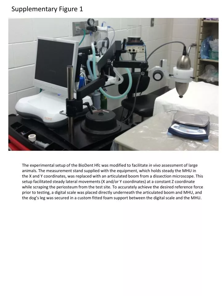
Supplementary Figure 1 The experimental setup of the BioDentHfc was modified to facilitate in vivo assessment of large animals. The measurement stand supplied with the equipment, which holds steady the MHU in the X and Y coordinates, was replaced with an articulated boom from a dissection microscope. This setup facilitated steady lateral movements (X and/or Y coordinates) at a constant Z coordinate while scraping the periosteum from the test site. To accurately achieve the desired reference force prior to testing, a digital scale was placed directly underneath the articulated boom and MHU, and the dog’s leg was secured in a custom fitted foam support between the digital scale and the MHU.
Suppl Figure 3 STEP BY STEP PROCESS OF THE MATLAB CODE CURVES ARE DEFINED USING FORCE-TIME DATA -The offset is fixed by adding the absolute value of the first point to the force array -The force and distance data is smoothed using Savitzky-Golay filtering method with polynomial order 3 and frame size of 51 -The derivative of each point in the force array is calculated to determine the slope TOUCHDOWN POINT DETERMINATION -The 1st cycle starting point is defined as the last point in the first 7% of the force derivative that has a value less than 0.002 DEFINING EACH CYCLE -The end of each cycle / beginning of the next cycle (local minima) is defined as the point that is less than the 150 points before it and the 150 points after it. -The final point (end of last cycle) is the last point where the force is greater than the average of the forces at the local minima -The dataset is then divided into cycles DEFINING CREEP INDENTATION DISTANCE -The first point of the creep region is defined as the first portion of the force that has a derivative less than 0.001 -The last point in the creep region is defined as the point where the the distance is at a maximum (determined using the Distance-Time graph). -This is repeated for each cycle
SupplFigure 3 cont. STEP BY STEP PROCESS OF THE MATLAB CODE (Cont.) CALCULATION OF CYCLE-BY-CYCLE DATA -This is done using both Distance vs. Time and Force vs. Distance plots. DISTANCEversus TIME This graph is used to calculate: - CID: Creep Indentation Distance - ID: Indentation Distance - IDI: Indentation Distance Increase -TID: Total Indentation Distance FORCE versus DISTANCE This graph is used to calculate -Energy: Area under the curve -US: Unloading Slope
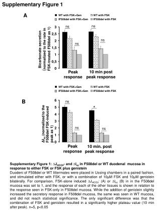
Supplementary Figure 4 A B C