Download
1 / 44
440 likes | 516 Views
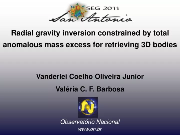
Radial gravity inversion constrained by total anomalous mass excess for retrieving 3D bodies. Vanderlei Coelho Oliveira Junior Valéria C. F. Barbosa. Observatório Nacional. www.on.br. Contents. Objective. 3D Gravity inversion method. Methodology.

E N D
Radial gravity inversion constrained by total anomalous mass excess for retrieving 3D bodies Vanderlei Coelho Oliveira Junior Valéria C. F. Barbosa Observatório Nacional www.on.br
Contents • Objective 3D Gravity inversion method • Methodology Do the gravity data have resolution to retrieve the 3D source? • Synthetic Data Inversion Result • Real Data Inversion Result • Conclusions
Objective Estimate from gravity data the geometry of an isolated 3D source Gravity data E N x y Source’s top 3D source Depth z
Methodology x Gravity observations y o N g Î R The 3D source has an unknown closed surface S. x y S Depth z 3D Source
Methodology x Gravity observations y o N g Î R Approximate the 3D source by a set of 3D juxtaposed prisms in the vertical direction. x y S Depth z 3D Source
Methodology x Gravity observations y o N g Î R We set the thicknesses and density contrasts of all prisms x y Depth z 3D Source
Methodology x Gravity observations y o N g Î R The polygon sides approximately describe the edges of a horizontal depth slice of the 3D source. The horizontal cross-section of each prism is described by an unknown polygon x y Depth z 3D Source
Methodology x Gravity observations y o N g Î R The polygon sides of an ensemble of vertically stacked prisms represent a set of juxtaposed horizontal depth slices of the 3D source. x y S Depth z 3D Source
Methodology x Gravity observations y o N g Î R The polygon sides of an ensemble of vertically stacked prisms represent a set of juxtaposed horizontal depth slices of the 3D source. x y Depth z
Methodology We expect that a set of juxtaposed estimated horizontal depth slices defines the geometry of a 3D source x y Depth z
Methodology ( ) x , y j j ( ) x , y j j The horizontal coordinates of the polygon vertices represent the edges of horizontal depth slices of the 3D source. x y Depth z
Methodology r ( ) , q r r r r r ) ) ) ) ) 3 , , , , , ( ( ( ( ( 3 q q q q q 8 5 6 7 4 r 4 6 8 7 5 ( ) , q 2 2 r ( ) , q 1 1 The polygon vertices of each prism are described by polar coordinates with an arbitrary origin within the top of each prism. x y Depth z Arbitrary origin
Methodology x y z k z , , i i i = q q z k k k T 1 [ ] q k L k m k k k k T [ r r x y ] ´ L = 1 M 1 M 1 ´ + 1 M 0 0 1 ( M 2 ) r ( ) , q k r r r r r ) ) ) ) ) 3 , , , , , ( ( ( ( ( 3 q q q q q m 6 8 7 5 4 r 4 6 5 8 7 ( ) , q 2 k 2 q r ( ) , q 1 1 The vertical component of the gravity field produced by the kth prism at the i th observation point (xi, yi, zi) is given by (Plouff, 1976) ( ) k f dz r g = , , , , , i x y Depth dz z
Methodology x y z k z , , i i i L å 1 k f = 1 k k m k q The gravity data produced by the set of L vertically stacked prisms at the i th observation point (xi, yi, zi) is given by ) g ( = dz r i , , , , , x y Depth z
Methodology r 1 r r r r 3 4 2 5 r r r 6 7 8 THE INVERSE PROBLEM Estimate the radii associated with polygon vertices and the horizontal Cartesian coordinates of the origin. x ( xo , yo ) y Depth z Arbitrary origin
Methodology y By estimating the radii associated with polygon vertices and the horizontal Cartesian coordinates of the arbitrary origin from gravity data, we retrieve a set of vertically stacked prisms x Gravity observations (xo , yo) x y Depth z 3D Source
The Inverse Problem 2 o - m g ( ) g 2 l G ( m ) ( m ) l å G ( ) m f = The constrained inversion obtains the geometry of 3D sourceby minimizing : m = + Parameter vector The constrained function The data-misfit function The constrained function G(m) is defined as a sum of several constraints:
The Inverse Problem » x y r r 1 1 r Depth r r r r 3 4 2 2 5 r r r 6 7 8 z Smoothness constraint on the adjacent radii defining the horizontal section of each vertical prism The first-order Tikhonov regularization on the radii of horizontally adjacent prisms This constraint favors solutions composed by vertical prisms defined by approximately circular cross-sections.
Inverse Problem » k r j r j r j + 1 k r j Smoothness constraint on the adjacent radii of the vertically adjacent prisms The first-order Tikhonov regularization on the radii of vertically adjacent prisms x y Depth z k k+1 This constraint favors solutions with a vertically cylindrical shape.
Inverse Problem x x x y y k +1 k +1 k+1 k+1 , , ( ( ) ) 0 0 0 0 x x , , y y k k k k ( ( ) ) 0 0 0 0 » y Depth z Smoothness constraint on the horizontal position of the arbitrary origins of the vertically adjacent prisms It imposes smooth horizontal displacement between all vertically adjacent prisms.
Inverse Problem z + z L . d z = o max The estimation of the depth of the bottom of the geologic body How do we choosezmax? Do the gravity data have resolution to retrieve the 3D source? The interpretation model implicitly defines the maximum depth to the bottom (zmax) of the estimated body by x y zo 1 . . . Depth dz L z max z
Inverse Problem g g g g Observed gravity data Observed gravity data Observed gravity data Fitted gravity data Fitted gravity data Fitted gravity data x x zo x zo zo zo zmax 1 mt zmax 2 zmax 3 zmax 4 z z s z The depth-to-the-bottom estimate of the geologic body 1) We assign a small value to zmax, setting up the firstinterpretation model. 2) We run our inversion method to estimate a stable solution 3) We compute the L1-norm of the data misfit(s)and the estimated total-anomalous mass ( mt ) Observed gravity data 4) We plot a point of the mt Xs-curve 5) We repeat this procedure for increasingly larger values of zmax of the interpretation model Fitted gravity data mtX s-curve x zmax 4 zmax 3 Optimum depth-to-bottom estimate zmax 2 zmax 1 z
Inverse Problem Observed gravity data g mt Fitted gravity data Estimated total-anomalous mass x zo s (mGal) z z Do the gravity data have resolution to retrieve the 3D source? mtX s-curve z Correct depth-to-bottom estimate L1-norm of the data misfit The gravity data are able to resolve the source’s bottom.
Inverse Problem Observed gravity data mtX s-curve Fitted gravity data g mt x Estimated total-anomalous mass zo z s (mGal) L1-norm of the data misfit z Do the gravity data have resolution to retrieve the 3D source? Minimum depth-to-bottom estimate z The gravity data are unable to resolve the source’s bottom.
INVERSION OF SYNTHETIC GRAVITY DATA
Synthetic Tests Two outcropping dipping bodies with density contrast of 0.5 g/cm³. Simulated shallow-bottomed body Maximum bottom depth of 3 km Simulated deep-bottomed body Maximum bottom depth of 9 km
Synthetic Tests Shallow-bottomed dipping body (true depth to the bottom is 3 km) The estimated total-anomalous mass ( mt )x the L1-norm of the data misfit (s) mtXs- curve zmax= 11.0 km 10 zmax= 2.0 km zmax= 3.0 km mt (kg x 1012) Estimated total-anomalous mass zmax= 1.0 km 5 0 0 0.4 0.2 s(mGal) L1-norm of the data misfit
Synthetic Tests zmax= 11.0 km 10 zmax= 2.0 km zmax= 3.0 km Depth (km) mt (kg x 1012) Estimated total-anomalous mass zmax= 1.0 km 5 0 x(km) y(km) 0.2 0.4 0 s(mGal) L1-norm of the data misfit Shallow-bottomed dipping body (true depth to the bottom is 3 km) mt Xs - curve True Body Initial guess
Synthetic Tests Depth (km) x(km) y(km) Shallow-bottomed dipping body (true depth to the bottom is 3 km) True Body Estimated body
Synthetic Tests Deep-bottomed dipping body (true depth to the bottom is 9.0 km) The estimated total-anomalous mass ( mt )x the L1-norm of the data misfit (s) mtXs- curve zmax= 9.0 km True depth to the bottom 25 zmax= 6.0 km Lower bound estimate of the depth to the bottom 20 15 mt (kg x 1012) Estimated total-anomalous mass 10 5 0 0.0 0.2 0.4 0.6 0.8 1.0 1.2 1.4 s(mGal) L1-norm of the data misfit
Synthetic Tests Deep-bottomed dipping body (true depth to the bottom is 9.0 km) By assuming two interpretation models with maximum bottom depths of 6 km and 9 km Lower bound estimate of the depth to the bottom (6 km) True depth to the bottom (9 km) 0 0 6 km 9 km Depth (km) 4.9 Depth (km) 4.9 9.9 9.9 x(km) x(km) y(km) y(km) True Body True Body Initial guess (6 km) Initial guess (9 km)
Synthetic Tests Deep-bottomed dipping body (true depth to the bottom is 9.0 km) By assuming two interpretation models with maximum bottom depths of 6 km and 9 km Lower bound estimate of the depth to the bottom (6 km) True depth to the bottom (9 km) 0 0 6 km 6 km 6 km 9 km Depth (km) 4.9 4.9 9.9 9.9 x(km) x(km) y(km) y(km) True Body True Body Estimated body Estimated body
INVERSION OF REAL GRAVITY DATA
Application to Real Data Real gravity-data set over greenstone rocks in Matsitama, Botswana. Study area
Application to Real Data Simplified geologic map of greenstone rocks in Matsitama, Botswana. (see Reeves, 1985)
Application to Real Data Gravity-data set over greenstone rocks in Matsitama (Botswana). 160 140 B 120 100 Northing (km) 80 60 A 40 20 20 40 60 80 100 120 Easting (km)
Application to Real Data The estimated total-anomalous mass ( mt )x the L1-norm of the data misfit (s) mtXs- curve zmax= 10 km zmax= 8 km mt (kg x 1012) Estimated total-anomalous mass zmax= 3.0 km s(mGal) L1-norm of the data misfit
Application to Real Data Estimated greenstone rocks in Matsitama (Botswana). Easting (km) Northing (km) N Depth (km) Estimated Body Initial guess
Application to Real Data Estimated greenstone rocks in Matsitama (Botswana). Easting (km) Northing (km) Easting (km) Northing (km)
Application to Real Data The fitted gravity anomaly produced by the estimated greenstone rock in Matisitama Northing (km) Easting (km)
Lower bound estimate of the depth to the bottom zmax= 6km mtXs- curve 25 0 Depth (km) 20 mt (kg x 1012) Estimated total-anomalous mass 15 Depth (km) 4.9 10 5 0 9.9 0.0 0.2 0.4 0.6 0.8 1.0 1.2 1.4 mtXs- curve s(mGal) L1-norm of the data misfit 10 zmax= 3.0 km mt (kg x 1012) Estimated total-anomalous mass 5 0 0.4 0.2 0 s(mGal) L1-norm of the data misfit Conclusions The proposed gravity-inversion method • Estimates the 3D geometry of isolated source • Introduces homogeneity and compactness constraints via the interpretation model • The solution depends on the maximum depth to the bottom assumed for the interpretation model. • To reduce the class of possible solutions, we use a criterion based on the curve of the estimated total-anomalous mass (mt) versus data-misfit measure (s). • The correct depth-to-bottom estimate of the source is obtained if the minimum of s on the mt × s curve is well defined Otherwise this criterion provides just a lower bound estimate of the source’s depth to the bottom.
Thank you for your attention