Download
1 / 41
510 likes | 722 Views
Local Search. CPSC 322 – CSP 5 Textbook §4.8 February 7, 2011. P.S. on Discussion of feedback. “Sometimes we don’t cover the full lecture” I vary the pace depending on class understanding Measured, e.g., by answers to coloured cards questions

E N D
Local Search CPSC 322 – CSP 5 Textbook §4.8 February 7, 2011
P.S. on Discussion of feedback • “Sometimes we don’t cover the full lecture” • I vary the pace depending on class understanding • Measured, e.g., by answers to coloured cards questions • I intentionally err on the side of preparing more material • If class understanding is unexpectedly good we’ll get through all slides • Typically, I don’t expect to cover everything! • Rather stop at a natural point, and continue next class • This way you also know what’s coming up next time • We are making good progress • We are one lecture ahead of last term’s schedule
Lecture Overview • Domain splitting: recap, more details & pseudocode • Local Search • Time-permitting: Stochastic Local Search (start)
Searching by domain splitting CSP, apply AC If domains with multiple values Split on one domain CSP1, apply AC CSPn, apply AC If domains with multiple values Split on one domain If domains with multiple values Split on one domain Recurse until no domains with multiple values Recurse until no domains with multiple values
Example “simple problem 2” in AIspace • 3 variables: A, B, C • Domains: all {1,2,3,4} • A=B, B=C, AC • We traced arc consistency + domain splittingfor this network last lecture
Arc consistency + domain splitting: example ({1,2,3,4}, {1,2,3,4}, {1,2,3,4}) 3 variables: A, B, C Domains: all {1,2,3,4} A=B, B=C, AC AC (arc consistency) ({1,2,3,4}, {1,2,3,4}, {1,2,3,4}) A ϵ {1,3} A ϵ {2,4} ({1,3}, {1,2,3,4}, {1,2,3,4}) ({2,4}, {1,2,3,4}, {1,2,3,4}) AC AC ({1,3}, {1,3}, {1,3}) ({2,4}, {2,4}, {2,4}) B ϵ {4} B ϵ {1} B ϵ {3} B ϵ {2} ({1,3}, {1}, {1,3}) ({1,3}, {3}, {1,3}) ({2,4}, {2}, {2,4}) ({2,4}, {4}, {2,4}) AC AC AC AC ({}, {}, {}) ({}, {}, {}) ({}, {}, {}) ({}, {}, {}) No solution No solution No solution No solution
Arc consistency + domain splitting: another example ({1,2,3,4}, {1,2,3,4}, {1,2,3,4}) 3 variables: A, B, C Domains: all {1,2,3,4} A=B, B=C, A=C AC (arc consistency) ({1,2,3,4}, {1,2,3,4}, {1,2,3,4}) A ϵ {1,3} A ϵ {2,4} ({1,3}, {1,2,3,4}, {1,2,3,4}) ({2,4}, {1,2,3,4}, {1,2,3,4}) AC AC ({1,3}, {1,3}, {1,3}) ({2,4}, {2,4}, {2,4}) B ϵ {4} B ϵ {1} B ϵ {3} B ϵ {2} ({1,3}, {1}, {1,3}) ({1,3}, {3}, {1,3}) ({2,4}, {2}, {2,4}) ({2,4}, {4}, {2,4}) AC AC AC AC ({1}, {1}, {1}) ({3}, {3}, {3}) ({2}, {2}, {2}) ({4}, {4}, {4}) Solution Solution Solution Solution
3rd formulation of CSP as search • Arc consistency with domain splitting • States: vector (D(V1), …, D(Vn)) of remaining domains, with D(Vi) dom(Vi) for each Vi • Start state: vector of original domains (dom(V1), …, dom(Vn)) • Successor function: • reduce one of the domains + run arc consistency • Goal state: vector of unary domains that satisfies all constraints • That is, only one value left for each variable • The assignment of each variable to its single value is a model • Solution: that assignment
Arc consistency with domain splitting algorithm(pseudocode for your Sudoku solver) • ProcedureAC_DS(V, dom,C, TDA) InputsV : a set of variables dom: a function such that dom(V) is the domain of variable V C: set of constraints to be satisfied • TDA: set of possibly arc inconsistent edges of the constraint networkOutputset of models of the CSP (empty if no model exists) • 1: dom ← GAC(V,dom,C,TDA) // run arc consistency initialized with TDA • 2: Ifdom includes an empty domain thenreturn {} • 3: If for all V1, …, Vn∈V, dom(Vi) has a single value vithen • 4: return the model {V1= v1, …, Vn= vn} • 5: Choose a variable V ∈ V • 6: [D1, …, Dn] ← Partition dom(V) into non-empty domains • 7: models ← {} • 8: for i=1, …, n do • 9: domi← dom with dom(V) replaced by Di • 10: TDA = {<Z, c> | Z∈V and Z ∈ scope(c) and V ∈ scope(c)} • 11:models ← models ∪ AC_DS(V, domi, C, TDA) • 12: return models Base case 1: no solution Base case 2: single model Domain splitting Arcs that could become inconsistent by reducing V’s domain.Z is some variable, c is some constraint involving both Z and V Recursive case
Learning Goals for arc consistency • Define/read/write/trace/debug the arc consistency algorithm. Compute its complexity and assess its possible outcomes • Define/read/write/trace/debug domain splitting and its integration with arc consistency
Lecture Overview • Domain splitting: recap, more details & pseudocode • Local Search • Time-permitting: Stochastic Local Search (start)
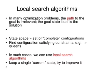
Local Search: Motivation • Solving CSPs is NP hard • Search space for many CSPs is huge • Exponential in the number of variables • Even arc consistency with domain splitting is often not enough • Alternative: local search • Often finds a solution quickly • But cannot prove that there is no solution • Useful method in practice • Best available method for many constraint satisfaction and constraint optimization problems • Extremely general! • Works for problems other than CSPs • E.g. arc consistency only works for CSPs
Some Successful Application Areas for Local Search Probabilistic Reasoning Propositionalsatisfiability (SAT) RNA structure design Scheduling of Hubble Space Telescope: 1 week 10 seconds University Timetabling Protein Folding
Local Search • Idea: • Consider the space of complete assignments of values to variables (all possible worlds) • Neighbours of a current node are similar variable assignments • Move from one node to another according to a function that scores how good each assignment is 1 8 1 4 8 3 4 3 5 2 8 1 4 8 3 4 3 5 7 7 7 7 4 5 7 1 2 8 6 4 5 7 1 2 8 6 3 7 3 4 1 3 3 7 3 4 1 3 8 7 2 8 8 7 2 8 9 9 5 4 3 8 7 2 5 4 3 8 7 2 4 7 1 2 8 5 6 4 7 1 2 8 5 6 1 1 8 8 7 5 8 4 8 6 7 3 5 7 5 8 4 8 6 7 3 5
Local Search Problem: Definition • Definition: Alocal search problem consists of a: • CSP: a set of variables, domains for these variables, and constraints on their joint values. A node in the search space will be a complete assignment to all of the variables. • Neighbour relation: an edge in the search space will exist • when the neighbour relation holds between a pair of nodes. • Scoring function: h(n), judges cost of a node (want to minimize) • - E.g. the number of constraints violated in node n. • - E.g. the cost of a state in an optimization context.
Example: Sudoku as a local search problem CSP: usual Sudoku CSP • One variable per cell; domains {1,…,9}; • Constraints: each number occurs once per row, per column, and per 3x3 box Neighbour relation: value of a single cell differs Scoring function: number of constraint violations 1 8 1 4 8 3 4 3 5 2 8 1 4 8 3 4 3 5 7 7 7 7 4 5 7 1 2 8 6 4 5 7 1 2 8 6 3 7 3 4 1 3 3 7 3 4 1 3 8 7 2 8 8 7 2 8 9 9 5 4 3 8 7 2 5 4 3 8 7 2 4 7 1 2 8 5 6 4 7 1 2 8 5 6 1 1 8 8 7 5 8 4 8 6 7 3 5 7 5 8 4 8 6 7 3 5
Search Space V1 = v1 ,V2 = v1 ,..,Vn = v1 V1 = v2,V2 = v1 ,..,Vn = v1 V1 = v1 ,V2 = vn,..,Vn = v1 V1 = v4,V2 = v1 ,..,Vn = v1 V1 = v4 ,V2 = v2,..,Vn = v1 V1 = v4 ,V2 = v1 ,..,Vn = v2 V1 = v4 ,V2 = v3,..,Vn = v1 Only the current node is kept in memory at each step. Very different from the systematic tree search approaches we have seen so far! Local search does NOT backtrack!
Iterative Best Improvement • How to determine the neighbor node to be selected? • Iterative Best Improvement: • select the neighbor that optimizes some evaluation function • Which strategy would make sense? Select neighbour with … • Evaluation function:h(n): number of constraint violations in state n • Greedy descent: evaluate h(n) for each neighbour, pick the neighbour n with minimal h(n) • Hill climbing: equivalent algorithm for maximization problems • Minimizing h(n) is identical to maximizing –h(n) Maximal number of constraint violations Similar number of constraint violations as current state No constraint violations Minimal number of constraint violations
Example: Greedy descent for Sudoku Assign random numbers between 1 and 9 to blank fields Repeat • For each cell & each number: Evaluate how many constraint violations changing the assignment would yield • Choose the cell and number that leads to the fewest violated constraints; change it Until solved 1 8 1 4 8 3 4 3 5 2 7 7 4 5 7 1 2 8 6 3 7 3 4 1 3 8 7 2 8 9 5 4 3 8 7 2 4 7 1 2 8 5 6 1 8 7 5 8 4 8 6 7 3 5
Example: Greedy descent for Sudoku Example for one local search step: Reduces #constraint violations by 3: • Two 1s in the first column • Two 1s in the first row • Two 1s in the top-left box 1 8 1 4 8 3 4 3 5 2 8 1 4 8 3 4 3 5 7 7 7 7 4 5 7 1 2 8 6 4 5 7 1 2 8 6 3 7 3 4 1 3 3 7 3 4 1 3 8 7 2 8 8 7 2 8 9 9 5 4 3 8 7 2 5 4 3 8 7 2 4 7 1 2 8 5 6 4 7 1 2 8 5 6 1 1 8 8 7 5 8 4 8 6 7 3 5 7 5 8 4 8 6 7 3 5
General Local Search Algorithm Random initialization Local search step
General Local Search Algorithm Based on local information. E.g., for each neighbour evaluate how many constraints are unsatisfied.Greedy descent: select Y and V to minimize #unsatisfied constraints at each step
Another example: N-Queens • Put n queens on an n × n board with no two queens on the same row, column, or diagonal (i.e attacking each other) • Positions a queencan attack
Example: N-queens h = ? h = 5 h = ? 0 2 3 1
Example: N-Queens 5 steps h = 17 h = 1 Each cell lists h (i.e. #constraints unsatisfied) if you move the queen from that column into the cell
The problem of local minima • Which move should we pick in this situation? • Current cost: h=1 • No single move can improve on this • In fact, every single move only makes things worse (h 2) • Locally optimal solution • Since we are minimizing: local minimum
Local minima Local minima • Most research in local search concerns effective mechanisms for escaping from local minima • Want to quickly explore many local minima: global minimum is a local minimum, too Evaluation function Evaluation function B State Space (1 variable) State Space (1 variable)
Different neighbourhoods • Local minimia are defined with respect to a neighbourhood. • Neighbourhood: states resulting from some small incremental change to current variable assignment • 1-exchange neighbourhood • One stage selection: all assignments that differ in exactly one variable. How many of those are there for N variables and domain size d? • O(dN). N variables, for each of them need to check d-1 values • Two stage selection: first choose a variable (e.g. the one in the most conflicts), then best value • Lower computational complexity: O(N+d). But less progress per step • 2-exchange neighbourhood • All variable assignments that differ in exactly two variables. O(N2d2) • More powerful: local optimum for 1-exchange neighbourhood might not be local optimum for 2-exchange neighbourhood O(dN) O(Nd) O(N+d) O(Nd)
Different neighbourhoods • How about an 8-exchange neighbourhood? • All minima with respect to the 8-exchange neighbourhood are global minima • Why? • How expensive is the 8-exchange neighbourhood? • O(N8d8) • In general, N-exchange neighbourhood includes all solutions • Where N is the number of variables • But is exponentially large
Lecture Overview • Domain splitting: recap, more details & pseudocode • Local Search • Time-permitting: Stochastic Local Search (start)
Stochastic Local Search • We will use greedy steps to find local minima • Move to neighbour with best evaluation function value • We will use randomness to avoid getting trapped in local minima
General Local Search Algorithm Extreme case 1: random sampling.Restart at every step: Stopping criterion is “true” Random restart
General Local Search Algorithm Extreme case 2: greedy descentOnly restart in local minima: Stopping criterion is “no more improvement in eval. function h”)
Greedy descent vs. Random sampling • Greedy descent is • good for finding local minima • bad for exploring new parts of the search space • Random sampling is • good for exploring new parts of the search space • bad for finding local minima • A mix of the two can work very well
Greedy Descent + Randomness • Greedy steps • Move to neighbour with best evaluation function value • Next to greedy steps, we can allow for: • Random restart: reassign random values to all variables (i.e. start fresh) • Random steps: move to a random neighbour
Which randomized method would work best in each of the these two search spaces? Evaluation function Evaluation function B A State Space (1 variable) State Space (1 variable) Hill climbing with random steps best on A Hill climbing with random restart best on B Hill climbing with random steps best on B Hill climbing with random restart best on A equivalent
Evaluation function Evaluation function B A Hill climbing with random steps best on B Hill climbing with random restart best on A State Space (1 variable) State Space (1 variable) • But these examples are simplified extreme cases for illustration, in reality you don’t know how you search space looks like • Usually integrating both kinds of randomization works best
Stochastic Local Search for CSPs • Start node: random assignment • Goal: assignment with zero unsatisfied constraints • Heuristic function h: number of unsatisfied constraints • Lower values of the function are better • Stochastic local search is a mix of: • Greedy descent: move to neighbor with lowest h • Random walk: take some random steps • Random restart: reassigning values to all variables
Stochastic Local Search for CSPs: details • Examples of ways to add randomness to local search for a CSP • In one stage selection of variable and value: • instead choose a random variable-value pair • In two stage selection (first select variable V, then new value for V): • Selecting variables: • Sometimes choose the variable which participates in the largest number of conflicts • Sometimes choose a random variable that participates in some conflict • Sometimes choose a random variable • Selecting values • Sometimes choose the best value for the chosen variable • Sometimes choose a random value for the chosen variable
Learning Goals for local search (started) • Implement local search for a CSP. • Implement different ways to generate neighbors • Implement scoring functions to solve a CSP by local search through either greedy descent or hill-climbing. • Implement SLS with • random steps (1-stage, 2-stage versions) • random restart • Local search practice exercise is on WebCT • Assignment #2 will be available on WebCT later today(due Wednesday, Feb 23rd) • Coming up: more local search, Section 4.8